 Genome Biology (2006): EGASP: The human ENCODE GENOME ANNOTATION ASSESSMENT PROJECT
SUPPLEMENTARY MATERIALS FOR
EGASP: The human ENCODE GENOME ANNOTATION ASSESSMENT PROJECT
R. Guigó +@, P. Flicek +, J. F. Abril +, A. Reymond, J. Lagarde, F. Denoeud,
S. Antonarakis, M. Ashburner, V. B. Bajic, E. Birney, R. Castelo, E. Eyras,
C. Ucla, T. R. Gingeras, J. Harrow, T. Hubbard, S. Lewis and M. Reese +@.
Genome Biology, 7(Suppl 1):S2,
2006.
[PubMed] [Full Text] [PDF] [Datasets]
+ These authors contributed equally to this work.
@ To whom correspondence should be addressed.
R. Guigó and M. Reese.
NEW We are pleased to announce that the EGASP Genome Biology supplement is now available via AMAZON. NEW
Contents
Summary
Different evaluation programs were used to compare the accuracy of the gene predictions submitted to the GENCODE EGASP'05 workshop, held at the Sanger Center on May 6-7, 2005. The results from those evaluations are provided here, along with some discussion on the different methods to calculate the accuracies of each different approach at three levels of the gene structure (basically at nucleotide, exon, transcript/gene levels).
Havana Curated Datasets
Files for each annotation freeze are available at the following ftp repository:
For the EGASP'05 workshop evaluations, the April 29th, 2005, freeze (version00.2_29apr05) was used. All the comparisons were calculated on ENCODE regions relative coordinates. The CDS exon predictions were evaluated against the annotations in the genes_with_cds subdirectory. Complete gene predictions (without distinguishing between UTR/CDS exons) were compared with the annotations from the genes_known_validated subdirectory. For some of the evaluation procedures, a nucleotide or an exon projection was required. The same transformations were performed onto the predicted genic structures and the curated ones. Those modifications are described in more detail in the corresponding methods section.
The following description of the annotation datasets was adapted from an email by France Denoeud.
Reference Annotation
The file to consider as the reference annotation is 44regions_genes.gtf.gz. It contains HAVANA-GENCODE annotations belonging to the following categories:
- Known
- Known protein coding genes (referenced in Entrez Gene, NCBI).
- Novel_CDS
- Novel protein coding genes annotated by Havana (not referenced in Entrez Gene, NCBI).
- Novel_transcript_gencode_conf
- Novel transcripts annotated by Havana (no ORF assigned) with at least one junction validated by RT-PCR.
- Putative_gencode_conf
- Putative transcripts (similar to novel transcripts, EST supported, short, no viable ORF) with at least one junction validated by RT-PCR. It also contains exons pairs from predictions that have been validated by RT-PCR.
This annotation is the most complete annotation of the ENCODE regions. It includes REFSEQ and ENSEMBL but contains much more, especially in terms of alternative splicing. We refer this set as the Genes set.
Coding Features Annotation
For the genes described above, some coding and non coding transcripts were annotated. The non coding transcripts are more dubious than the coding ones, as no ORF could be determined without ambiguity (and some of the non coding transcripts can be partial). If we need to be more conservative, we might want to use the file 44regions_coding.gff.gz. It contains only the coding transcripts from HAVANA-GENCODE Known and Novel_CDS categories (with coding and non coding exons, the other categories from the previous section are non coding). We refer this set as the Coding Genes set.
Annotation Statistics
On the set Coding Genes set there are 439 genes, 2431 transcripts, 17520 exons and 9530 coding exons. On the set Genes there are 551 genes, 2603 transcripts, 18074 exons and 9530 coding exons (as already said in the previous section, set Genes contains set Coding Genes). It can be seen from those figures that the number of coding exons was the same (and they are also the same at the coordinates level). Furthermore, there was only around 7% more untranslated exons.
Gene Finding Predictions Sets
Gene predictions were submitted under one of the seven categories described in the EGASP'05 workshop page. A table with the number of GTF features predicted on each ENCODE sequence can be downloaded from the following links: ordered by submitter code or ordered by prediction category.
Files Submitted to EGASP'05
All the submissions are available from the following link:
They were reformatted and renamed to made them more suitable for uploading into the ENCODE specific UCSC Genome Browser. In some cases the predictions on the test sequence set were asked for to the corresponding groups in order to show all the predictions on the complete set of 44 ENCODE regions. The new files can be found at:
Post-Submissions
There are four files under this category. They basically correspond to fixes on a previously submitted prediction set. For instance, initial GeneMark predictions were obtained on the unmasked sequences for the ENCODE regions. In this case, the post-submission contains the results for GeneMark on the properly masked sequences. On the other hand, Fgenesh predicted genes with Refseq support in reverse strand were shifted by 1 when they were transfered to GTF format. This was fixed on the latest Softberry submitted predictions.
The post-submissions are available from the following link:
Evaluation Methods
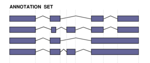 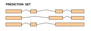 |
The two figures on the left sketch the exonic structure of a set of annotated and predicted transcripts for a given locus. You can obtain from here a PDF file summarizing all the figures for the nucleotide and exon level comparisons. The accuracy measures being used along this section are described in Burset and Guigó [Genomics, 34/3:353-357, 1996], Reese et al [Genome Research, 10/4:483-501, 2000] and Guigó et al [Genome Research, 10/10:1631-1642, 2000]. |
Comparisons at Nucleotide Level
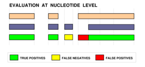 |
The genic structures shown in the previous section were projected onto a set of non-overlapping annotated/predicted nucleotide regions. Those regions were then compared as if they were single exons in order to calculate the corresponding Sn, Sp and CC measures. |
Comparisons at Exon Level
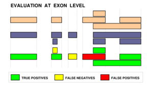 |
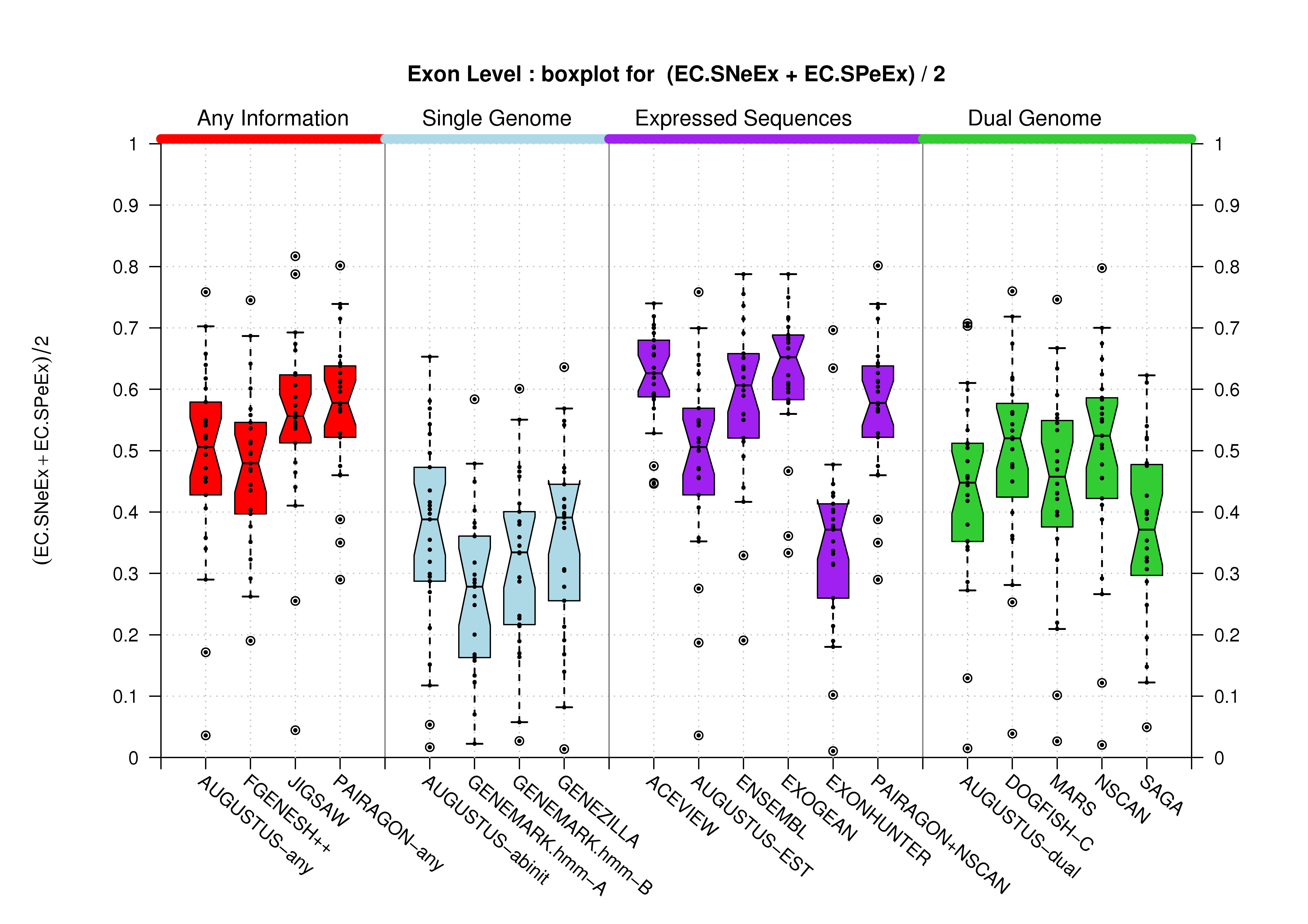
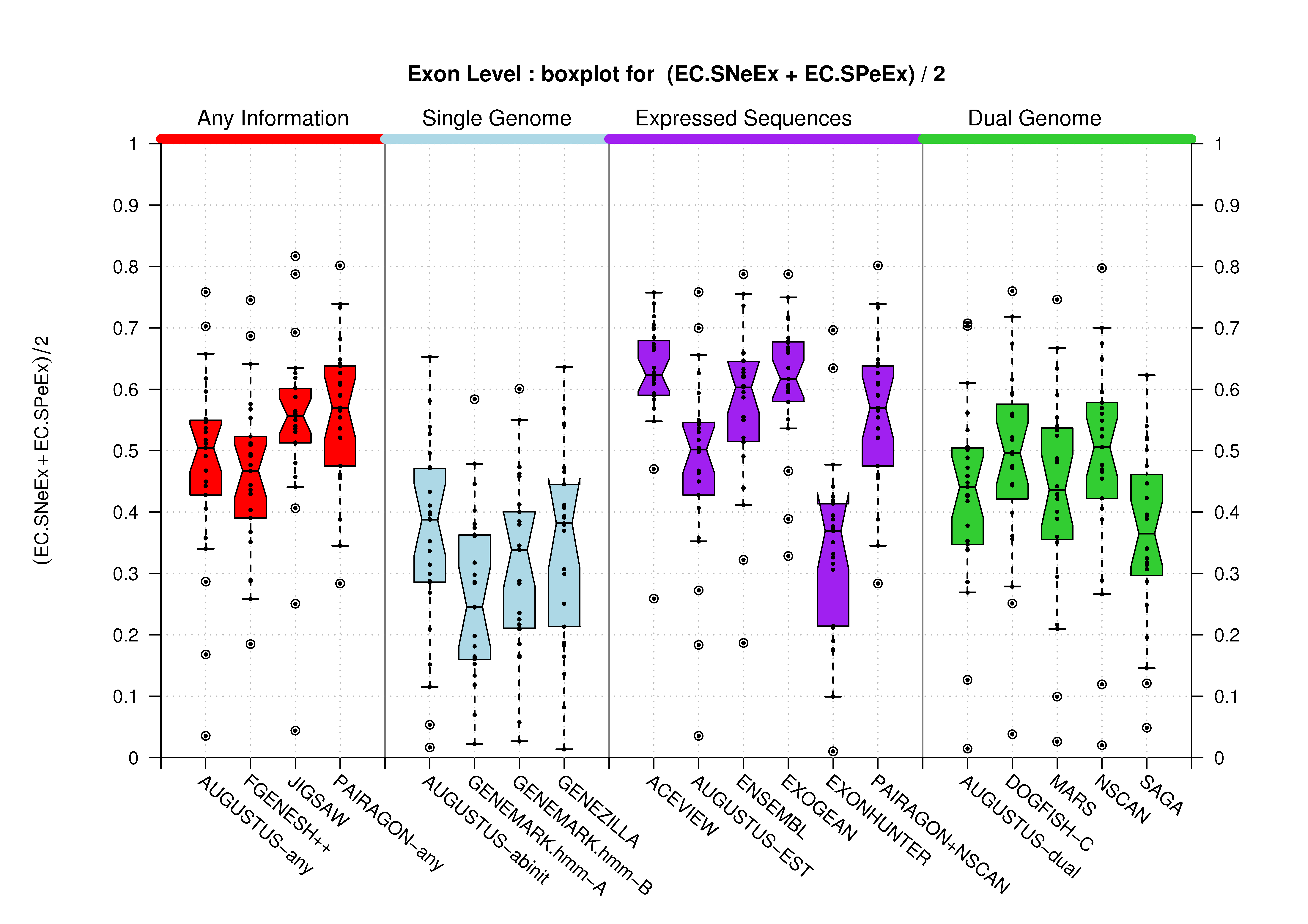
For each program all of the unique exons are determined and compared to the unique exons in the annotation. Sensitivity is defined as the fraction of the unique annotation exons that are predicted exactly by each program. Specificity is the fraction of each program's unique exons that are correct (i.e. match an annotation exon). Missed exons are the number of unique coding exons in the annotation that are not predicted exactly. Wrong exons are the total number of unique exons in the prediction that do not match any coding exon in the annotation. |
Exon Level Predictions: There are 4387 unique exons in the annotation and a total of 9180 coding exons in all annotated transcripts.
Corrections:
- The fgenesh++ predictions were resubmitted after the meeting to correct an off-by-one error in the creation of the gtf. The corrected predictions are included above. The original submission had exon sensitivity: 0.58537; exon specificity: 0.55309; missed exons: 1819; wrong exons: 2075; total exons: 5693; unique exons: 4643.
- The Exogean predictions presented at the meeting were not correct because of an error in the evaluation program. The correct statistics are posted here.
- The GeneMark-HMM predictions were inadvertently run on unmasked sequence. This leads to a large number of false positive predictions. Corrected predicted were submitted after the meeting, but the original predictions are reported here.
Comparisons at Gene/Transcript Level
 |
IMIM
To evaluate the accuracy of alternative splicing prediction, an evaluation perl script developed by Eduardo Eyras was used. He provided the following description of how different accuracy parameters are calculated by this tool. You can get in contact with him if you are interested to obtain a copy of this evaluation tool.
- Gene Level
- A gene is taken as a cluster of transcripts (according to exon-overlap) in the same strand. When we compare genes, we in fact compare clusters of transcripts.
At gene level we compare all the nucleotides in the prediction and in the annotation. We perform a projection of each set to the genome (to eliminate the redundant base-pairs), and compare the projections of the predictions and annotations.
We also compare the exons. Similarly to the nucleotide comparison, we extract the set of unique exons in the annotation and prediction sets (i.e. eliminate redundancy). We then compare the set of exons and label as found each exon that has been correctly predicted with both splice-sites correct.
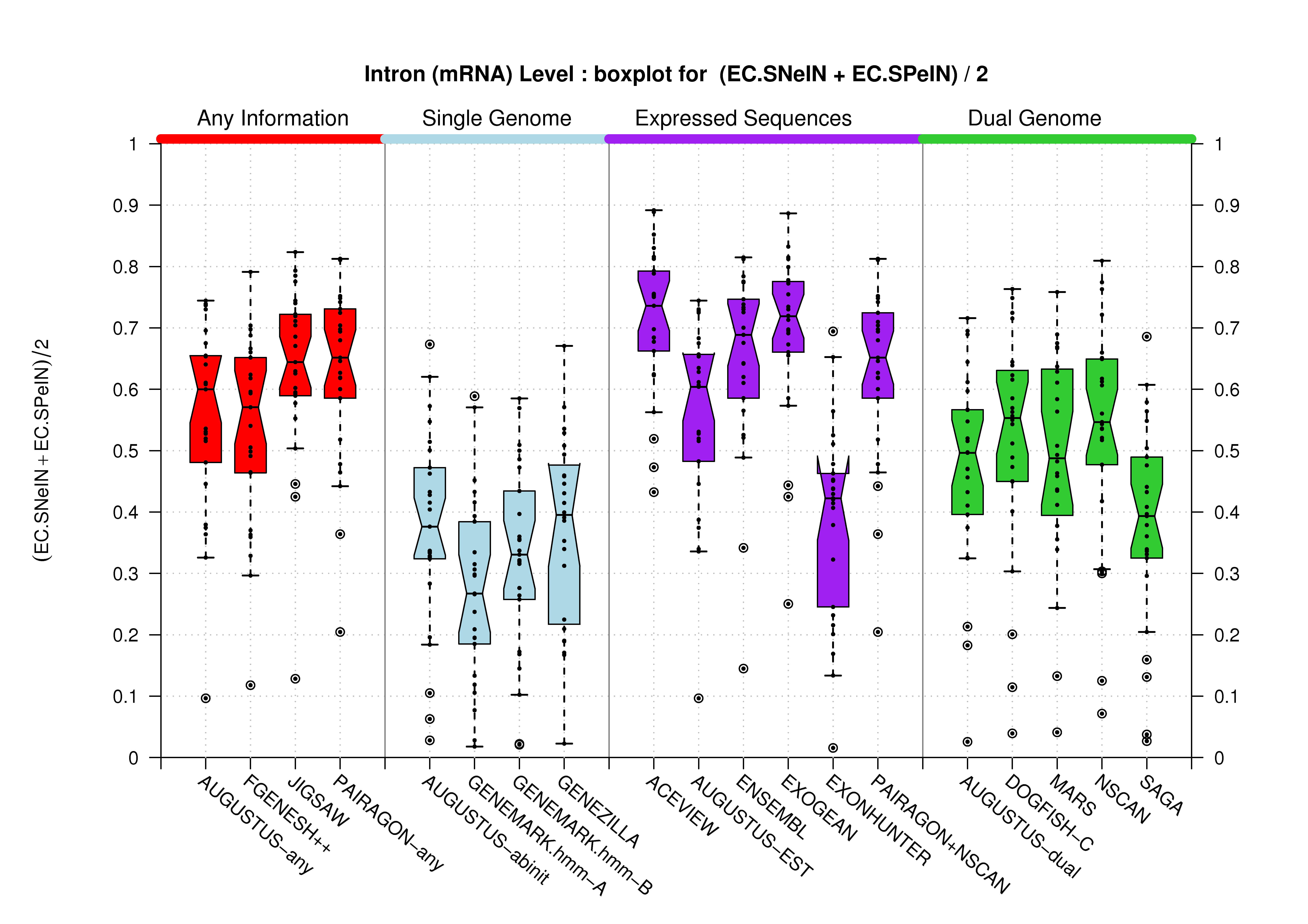
Likewise, we compare the set of unique introns in each gene prediction. We project all annotated and predicted introns into two sets of non-redundant introns (annotated and predicted), and compare these two sets regardless of the transcript to which they are associated to. For this comparison, only the actual boundaries of the intron (donor and acceptor sites) are used. This measure can give an estimate of the accuracy of the splice-site prediction.
These three measures, nucleotide, exon and intron level, give an overall measure of the accuracy, regardless of the actual transcript structures. For each of them we calculate the sensitivity (Sn), the specificity (Sp), the wrong cases (W), as the fraction of predictions that do not overlap any annotation, and the missing cases (M), as the fraction of annotations that do not overlap any prediction.
For every comparison of genes, we establish a one-to-one mapping of transcripts in the following way. For every possible pair of transcripts (one from the annotation and one from the prediction), we calculate the correlationa coefficient at the nucleotide level (CCn), where TN is calculated using the extension in the genome of these two transcripts only. The best possible pairs can be taken as a loose measure of accuracy at the transcript level. At this stage we also calculate the more strict measure related to the annotated transcripts which are exactily found by the annotation.
- Transcript level
- Once this one-to-one mapping of transcripts has been established we can produce measures at the transcript level, which gives a better view of the accuracy taking into account the connectivity of exons into splicing forms.
We calculate the same measures as above (SN, SP, W, M) for nucleotides, exons and introns, but this time, only using the transcript-pairs obtained by the method described above. These measures give a better estimate of the accuracy of the predicted exon-intron structures, whereas the gene-based comparisons described above provide an overall performance per gene locus.
All these measures are calculated per gene locus. Gene loci in the annotation and the prediction are grouped according to overlap, and the measures calculated for each group. Currently there is no measure of the split and joining of genes or transcripts.
A summary result is also obtained with the averaged measures. Besides these measures we also calculate the average exact transcripts found per gene-pair, as an estimator of how well multiple transcripts are found by the prediction.
EBI
Evaluations at the Transcript and the Gene level are meant to test the ability of the gene-prediction algorithms to correctly connect the predicted exons into transcription structures. Genes in the Havana annotation have an average of 2.53 (CHECK NUMBER) transcripts per gene. Most prediction programs are only able to predict on transcript per gene.
- Transcript Level
- Transcripts are defined by the prediction algorithm as the connection between the coding exons and generally run from a start codon to stop codon. Partial transcript predictions, such as those that might arise at the end of the ENCODE region, are also evaluated.
A transcript is judged to be correct if the start and stop codon locations are correctly predicted and the boundary of every coding exon is correct. Non-coding exons are not considered.
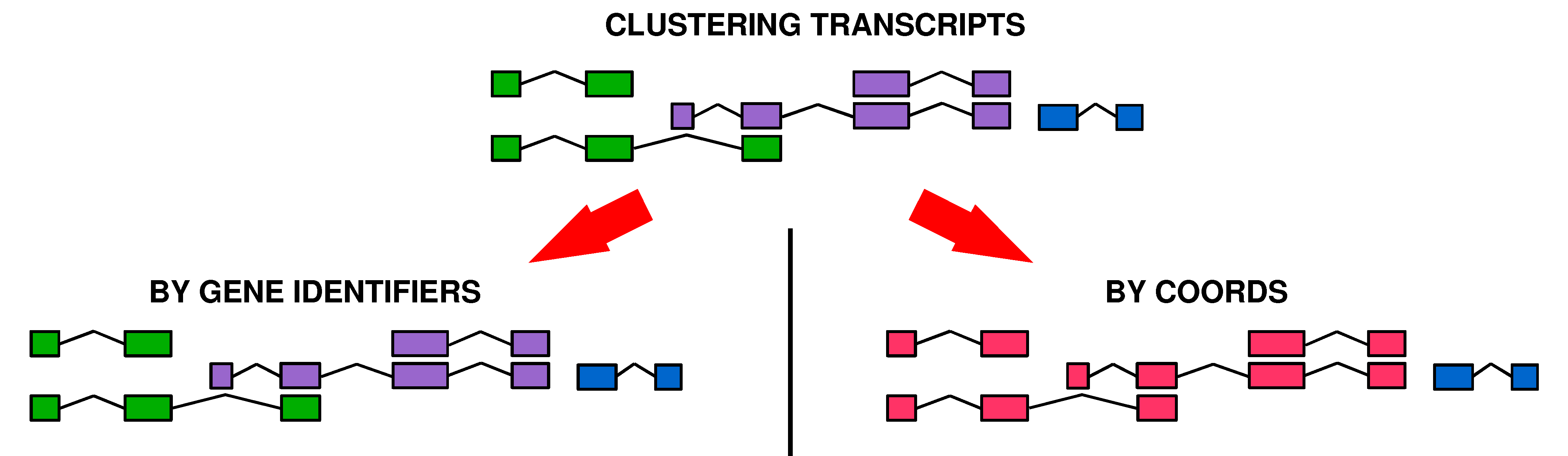
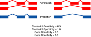
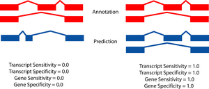
- Gene level
- A gene is judged to be correct if at least one of its transcripts is predicted correctly (as defined above). The following figures detail the relationship between gene and transcript level statistics for several example predictions.
 |
 |
 |
EGASP'05 Evaluation Results
Evaluations were obtained for each of the 44 ENCODE regions. Furthermore, annotations and predictions for those regions were grouped to evaluate the overall accuracy of the gene-finding tools in the following sets:
- EN_TRN13.- The 13 regions that were used for training all the gene-finding software, also known as the training set.
- EN_PRD31.- The 31 regions on which the predictions for the GENCODE workshop were made, also known as the test set.
- EN_ALL44.- A summary for all the ENCODE regions (in few cases incomplete because the submitters only provided the predictions for the test set).
- EN_MNL14.- The set of all manual sequence picks containing genes of interest.
- EN_RND30.- The set of all randomly choosen ENCODE sequences.
- EN_MNLp12.- Manual sequence picks from the predictions set.
- EN_RNDp19.- Randomly choosen sequences from the predictions set.
One of the advantages of grouping the annotations/predictions in the way shown above, is that the final evaluation takes into account those regions in which the programs predicted genes but there were no annotated genes and viceversa. Regions ENr112, ENr311 and ENr313, are a good example of sequences without manually-curated annotated genes for which some gene-finders produced predictions. Moreover, the multisequence sets are also usefull to detect possible biases on the accuracy of the predictions due to the samples being used.
Annotation for the following 13 regions was released before the workshop (i.e. these regions are considered the training set): ENm004, ENm006, ENr111, ENr114, ENr132, ENr222, ENr223, ENr231, ENr232, ENr323, ENr324, ENr333, ENr334. As noted above, these regions are not necessarily reflective of the entire set of ENCODE sequences.
The following files contain the complete set of measures computed at different levels, for each submission and each sequence, in plain ASCII tabular format. The column names from the first row of those tables are also described here.
| ANALYSIS SET | SCORES | DESCRIPTION | ||
|---|---|---|---|---|
| EBI on Havana Coding Genes Set | TBL | TXT | ||
| IMIM on Havana Coding Genes Set | TBL | TXT | ||
| IMIM on Havana Genes Set | TBL |
(Sn+Sp)/2 figures appearing on the paper were produced from the EBI data. The following sections provide the same analysis on the two datasets by IMIM, including analysis on more exonic features, such as splice sites. One column has been computed for the Coding Genes Havana set and the other column was derived from the Genes Havana set. For completeness shake, we include here the Genes evaluation. When comparing all the exons (coding and non-coding), any difference in the evaluation results can be due to the facts that the Genes set contains the Coding Genes set and that it includes 112 genes more (along with their corresponding 172 transcripts). Those genes are made of non-coding exons, thus major differences can be expected when comparing all predicted exons against all those annotated exons. However, the figures below show that the evaluation results are quite similar for the two annotation sets.
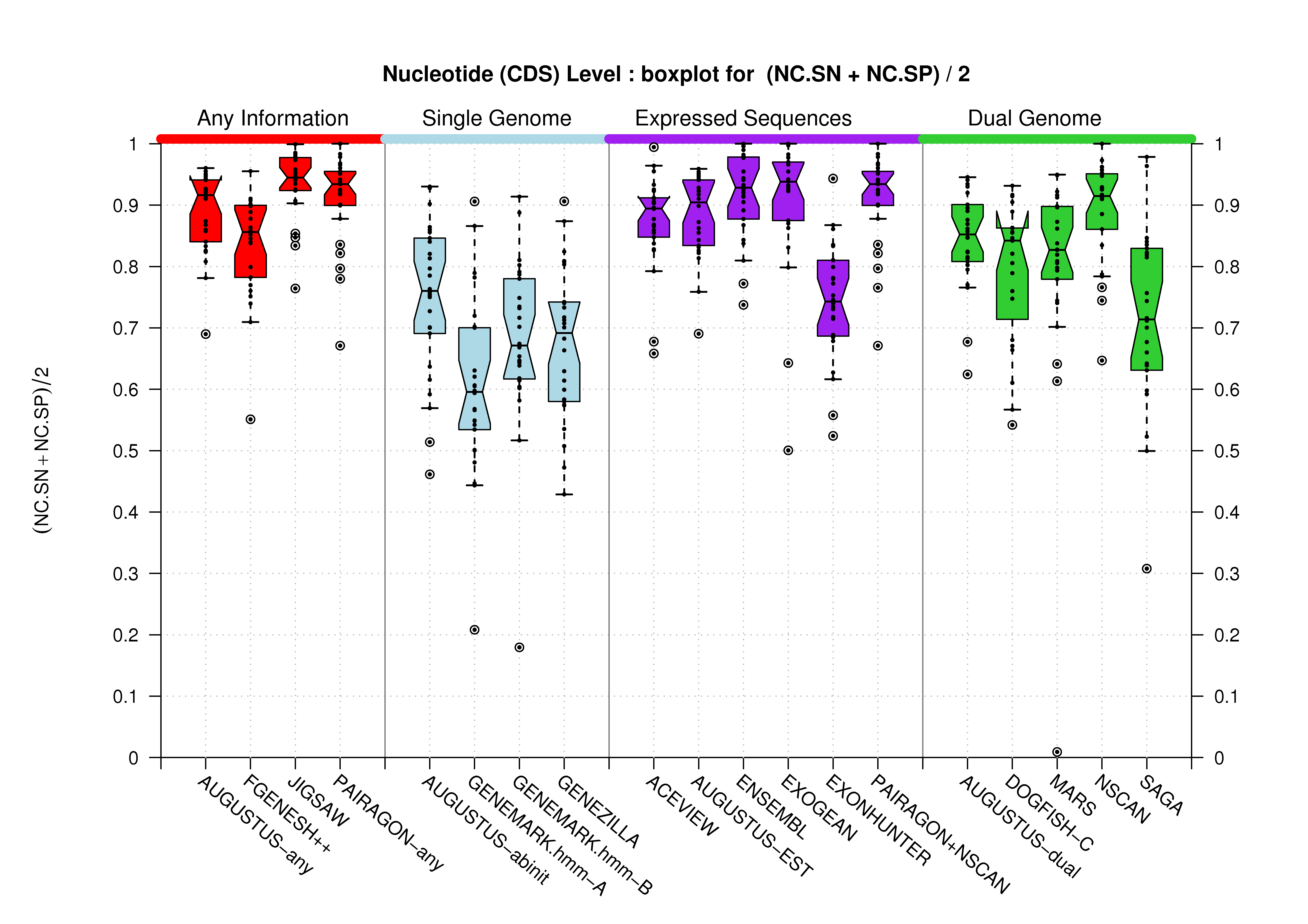
Nucleotide Level
| Feature | Havana Coding Genes Dataset | Havana Genes Dataset | |
|---|---|---|---|
| CDS | 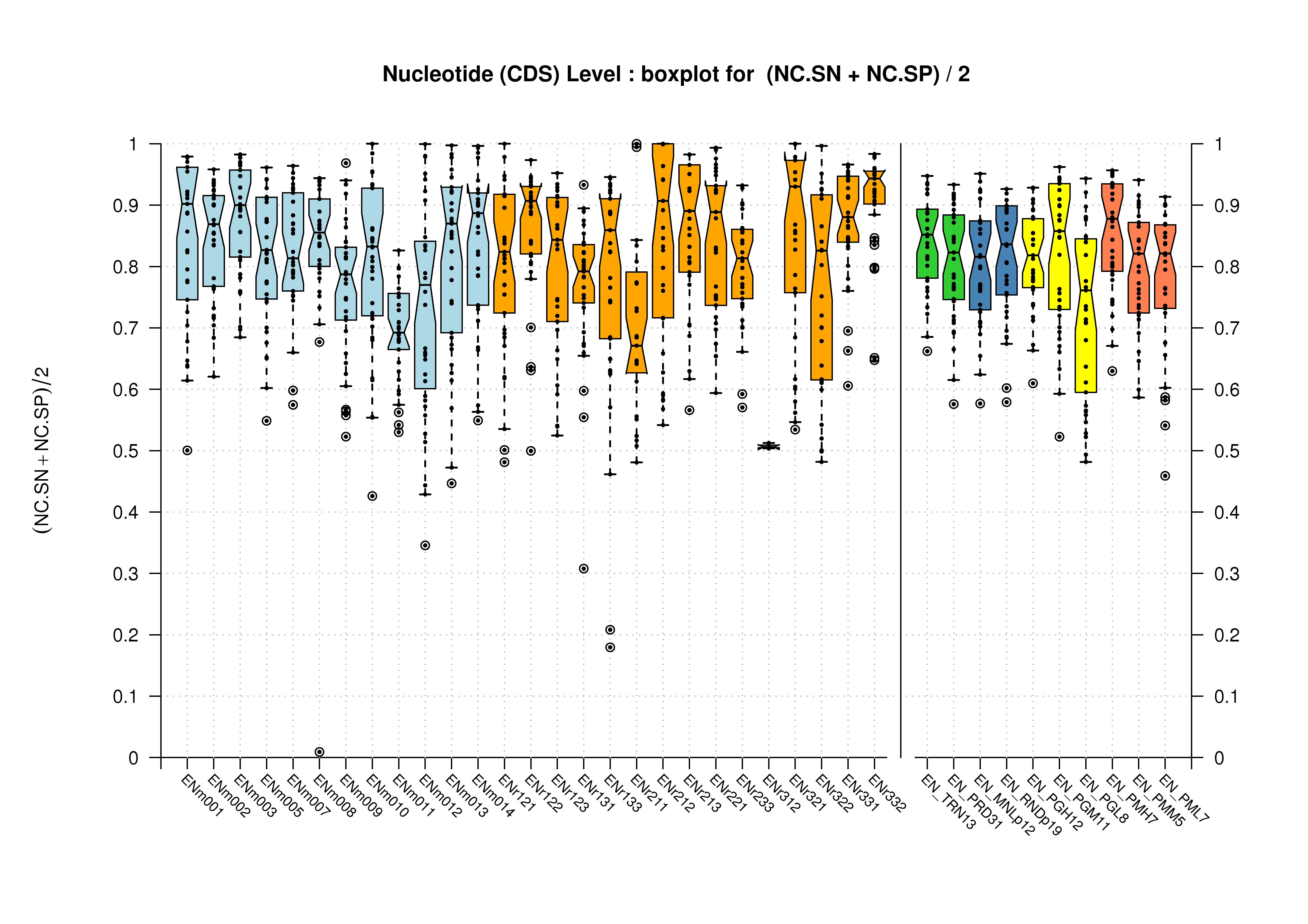 [PS][PDF][PNG] |
 [PS][PDF][PNG] |
 [PS][PDF][PNG] |
| mRNA | 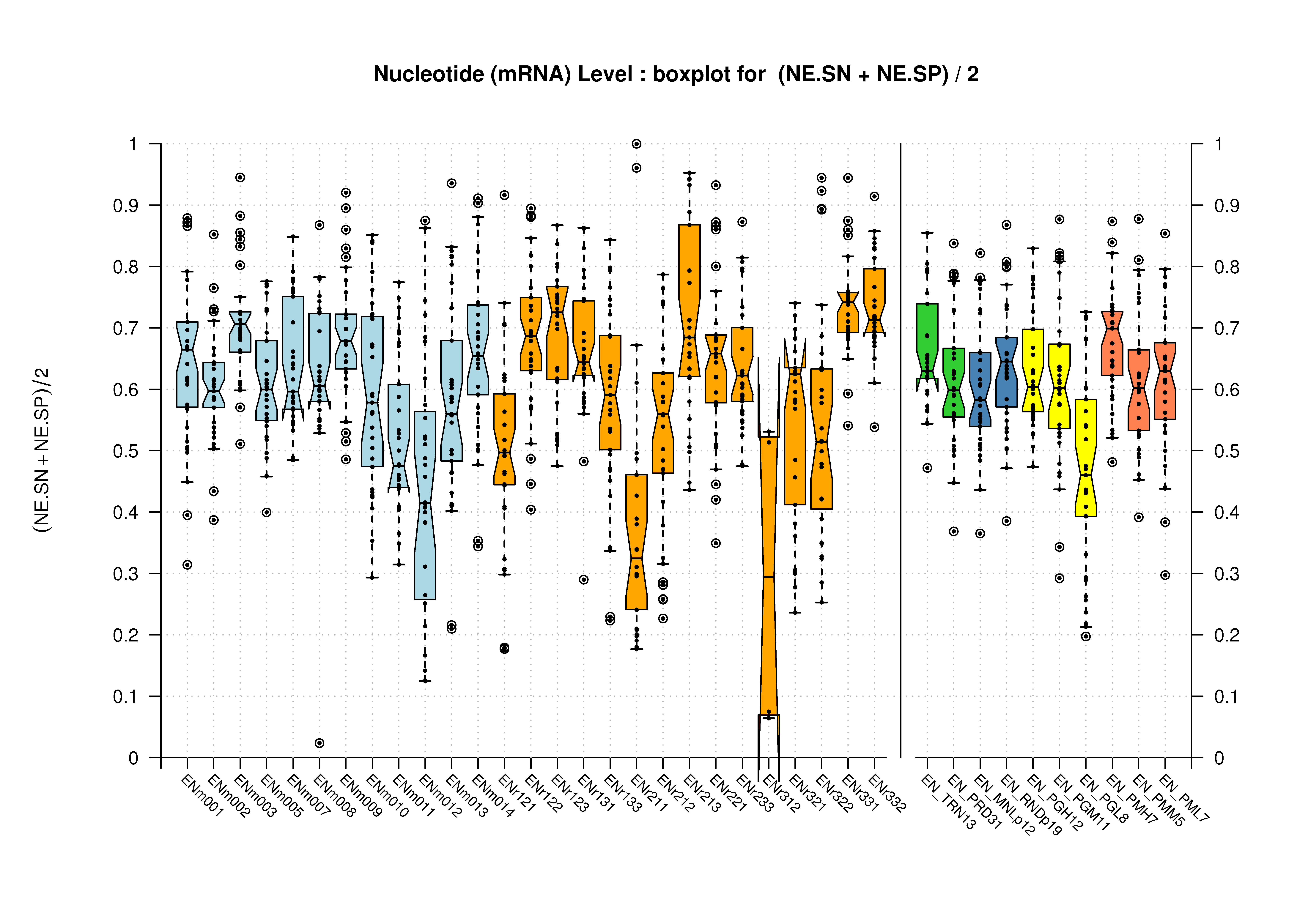 [PS][PDF][PNG] |
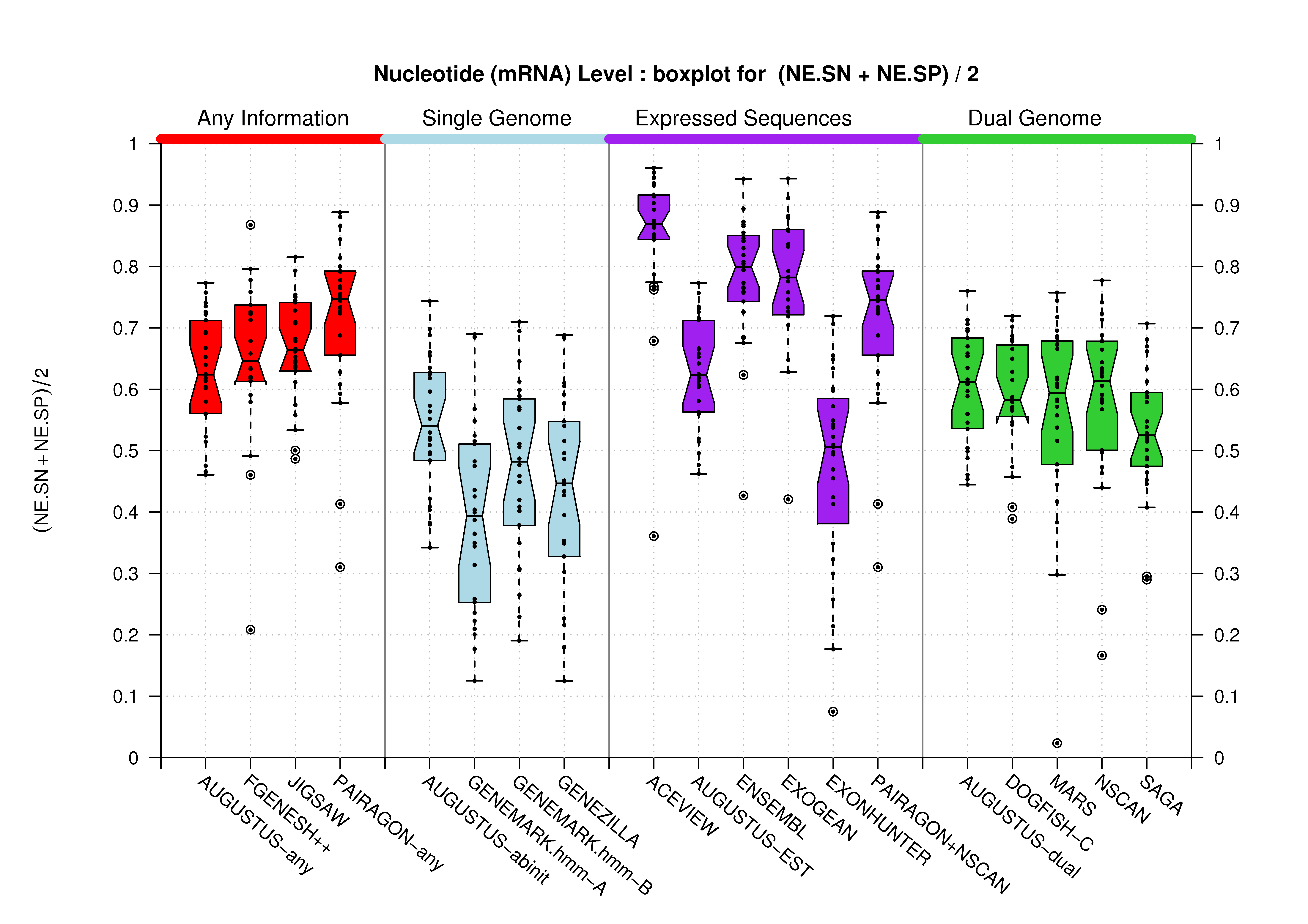 [PS][PDF][PNG] |
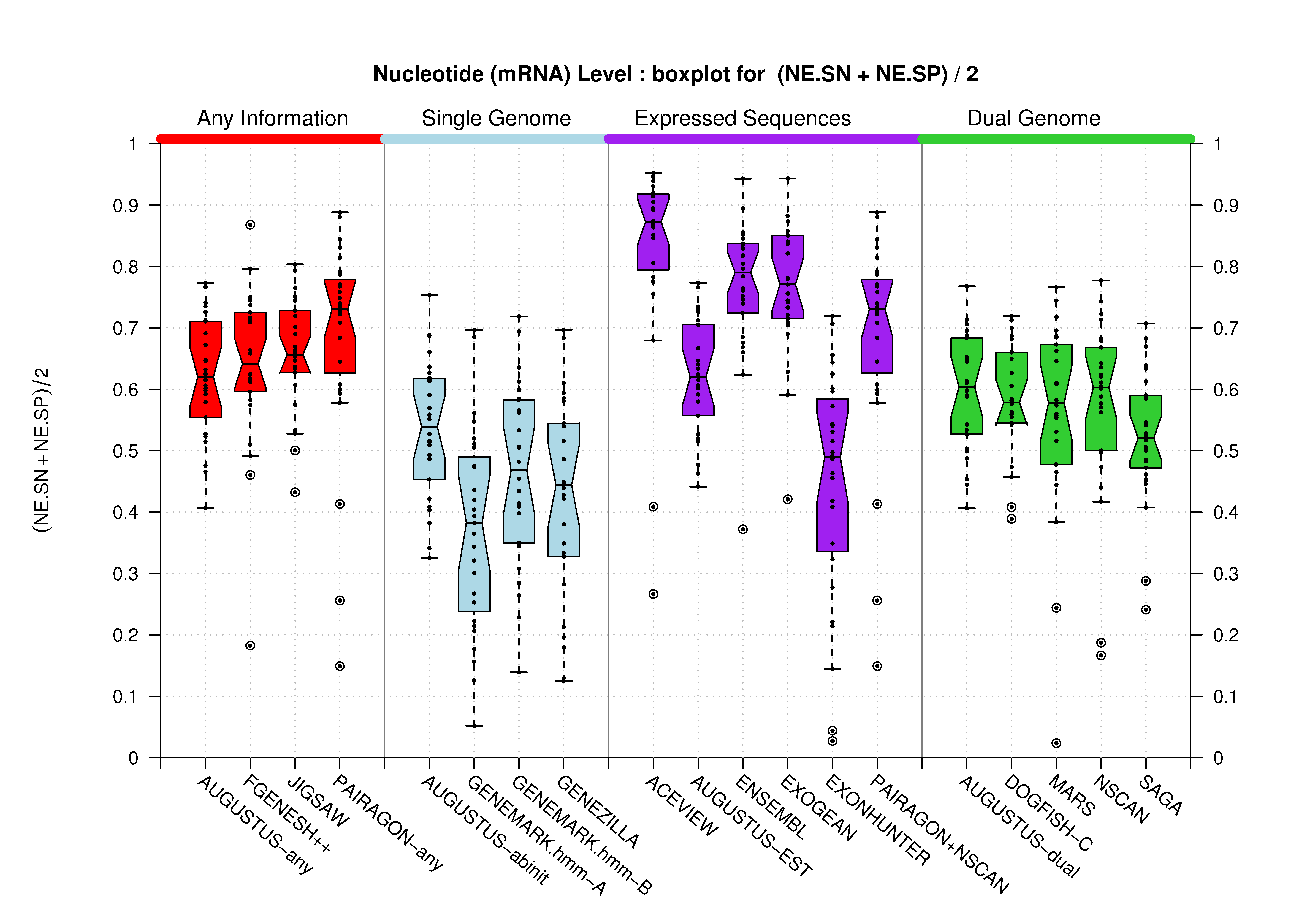 [PS][PDF][PNG] |
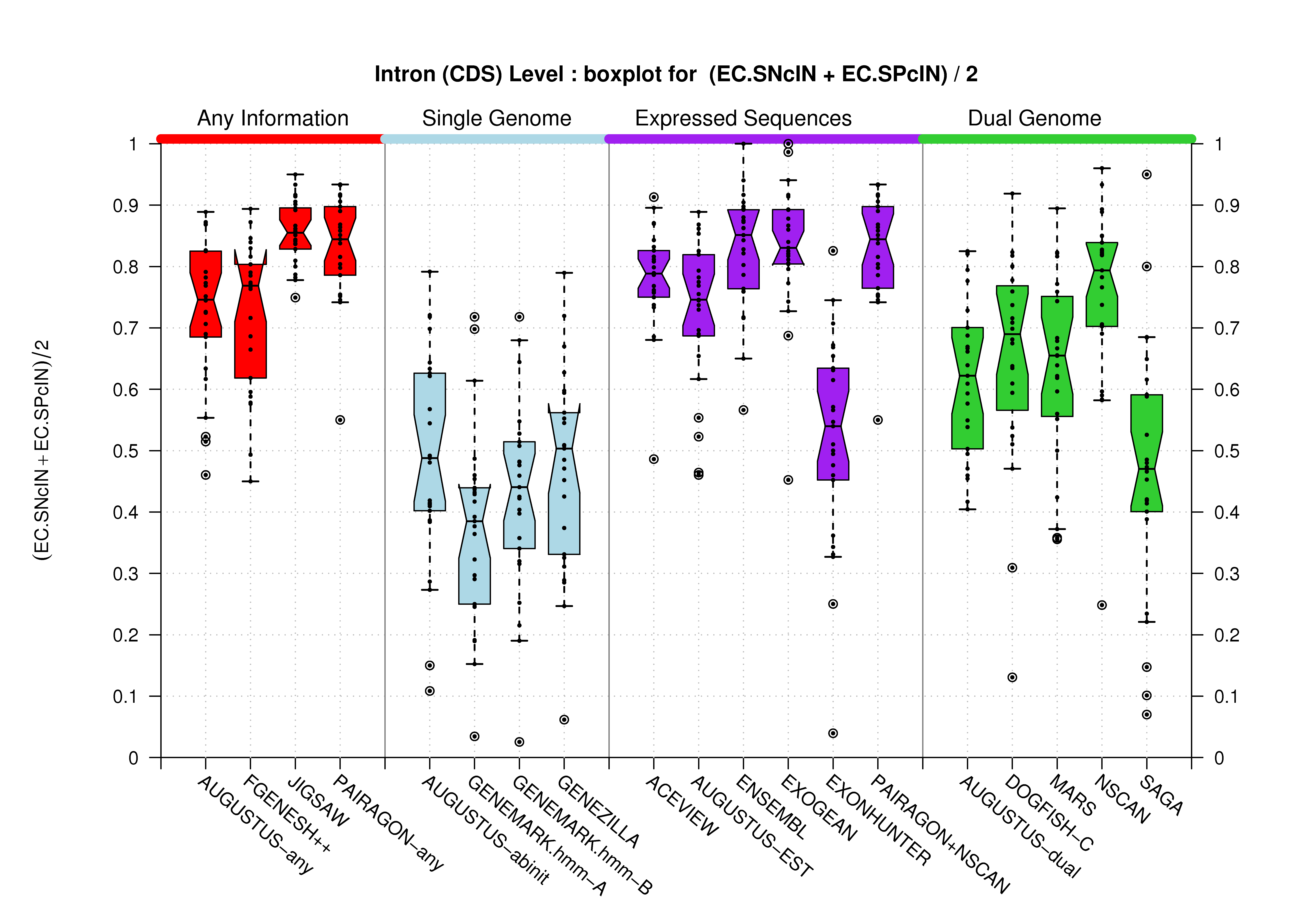
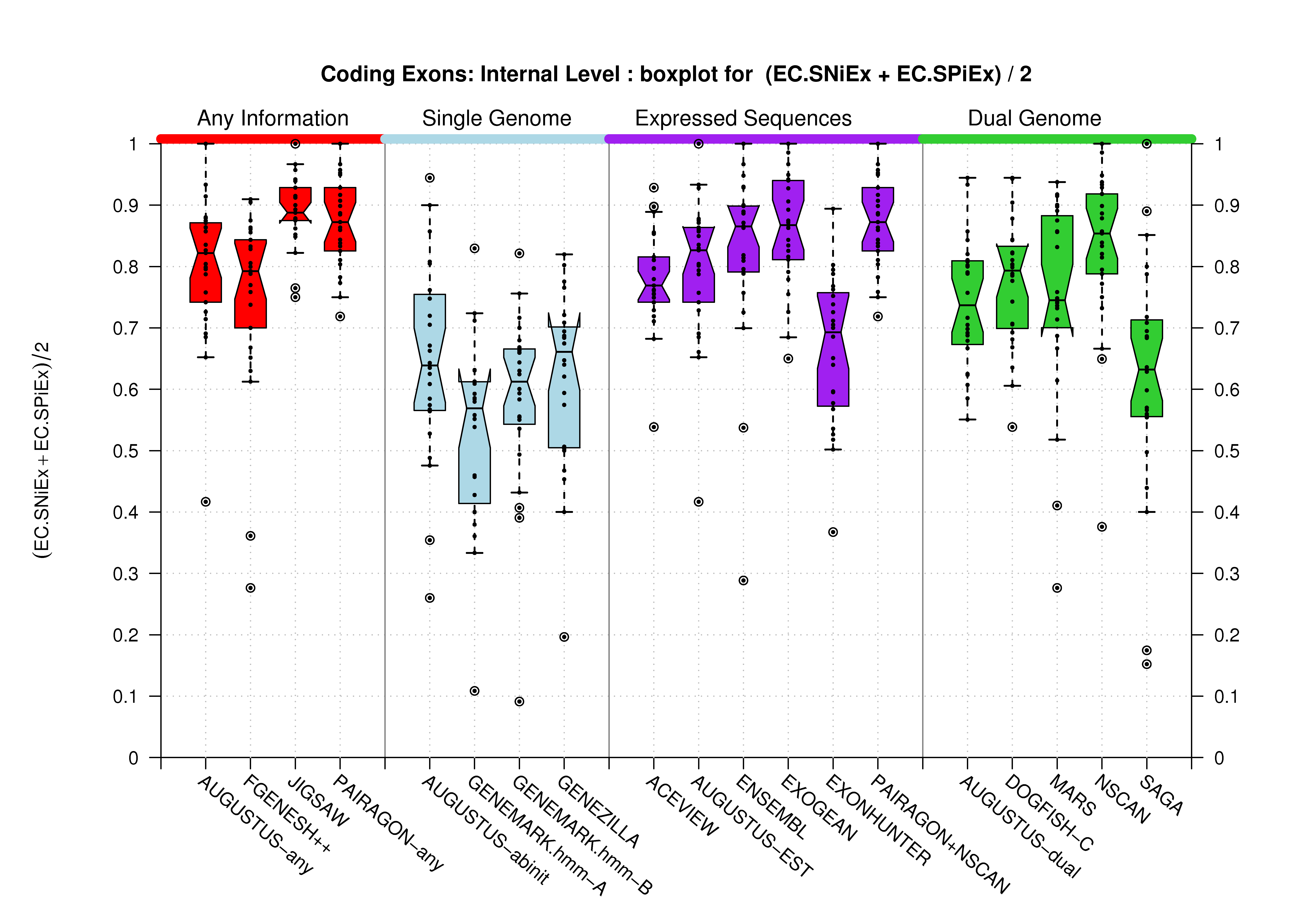
Coding Exon Level
It has been already stated and it can be observed in the previous section; at the coding features level, there are no differences between the evaluation results from comparing predictions against the Coding Genes or the Genes Havana datatsets. It has been explained in the Havana Curated Datasets section, that the Coding Genes dataset is a subset of the Genes one. Therefore, here you can only find the results for the first dataset.
| Feature | Havana Coding Genes Dataset | ||
|---|---|---|---|
| All Coding Exons | 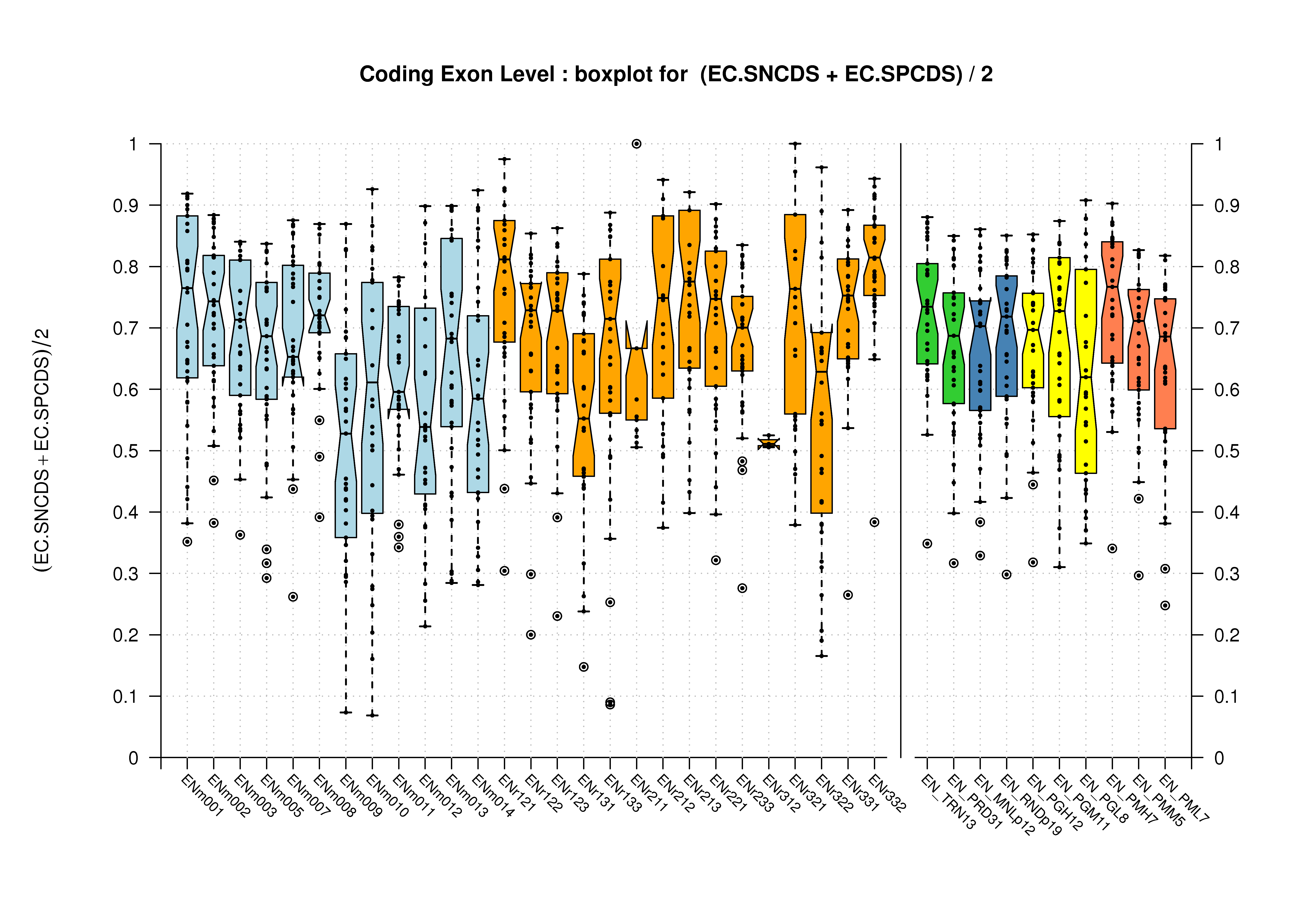 [PS][PDF][PNG] |
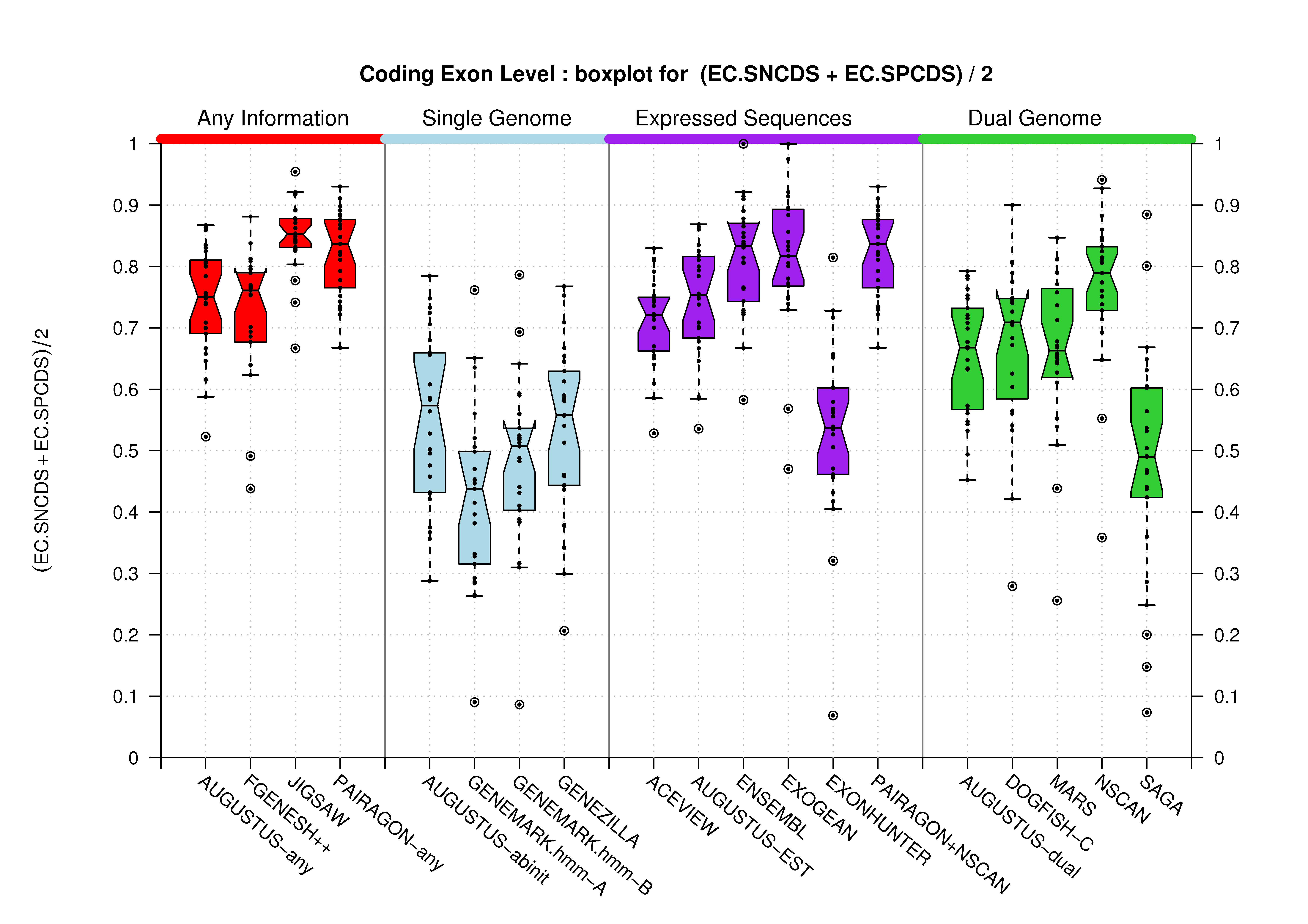 [PS][PDF][PNG] |
|
| Introns within Coding Exons |
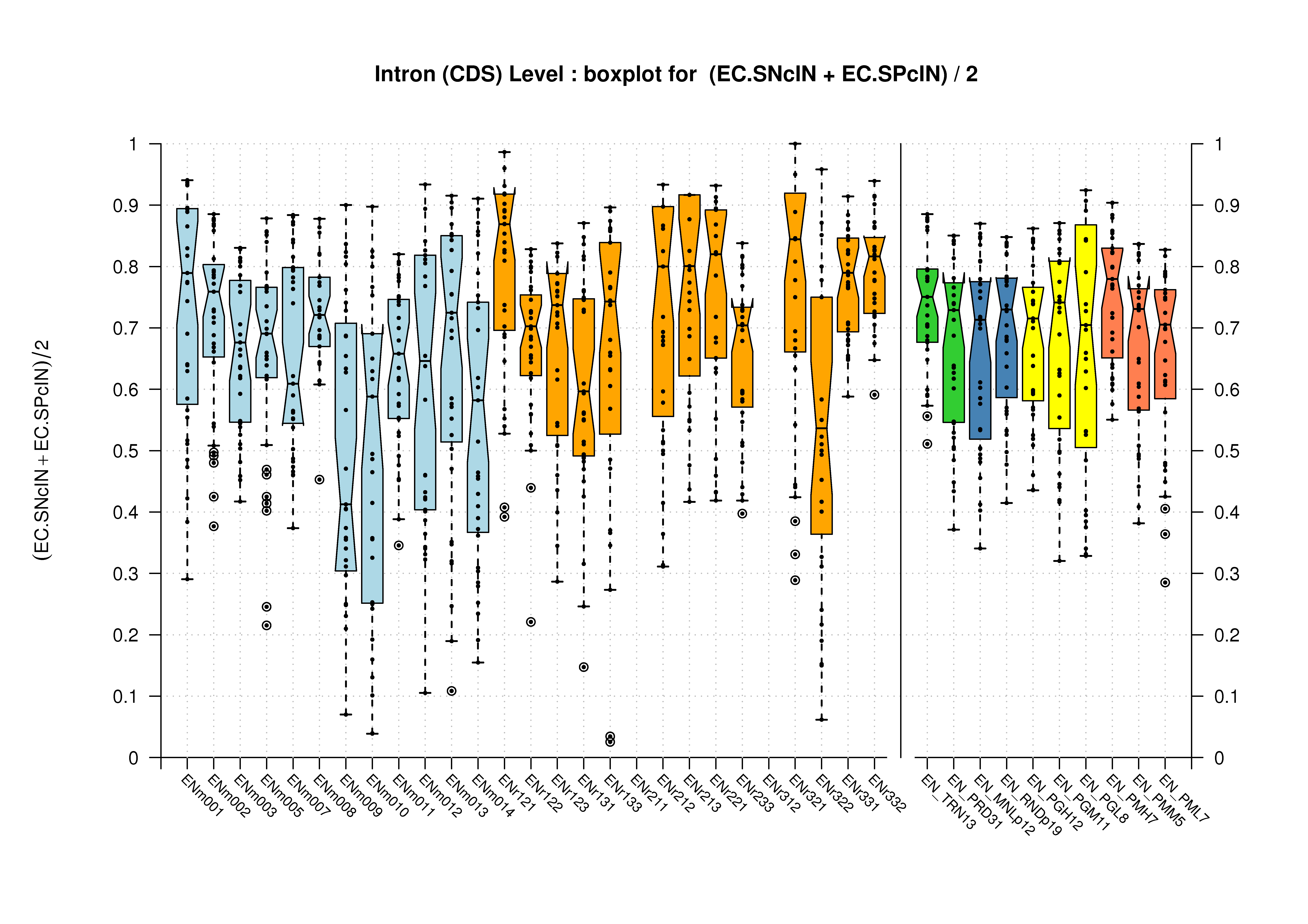 [PS][PDF][PNG] |
 [PS][PDF][PNG] |
|
| First Exon | 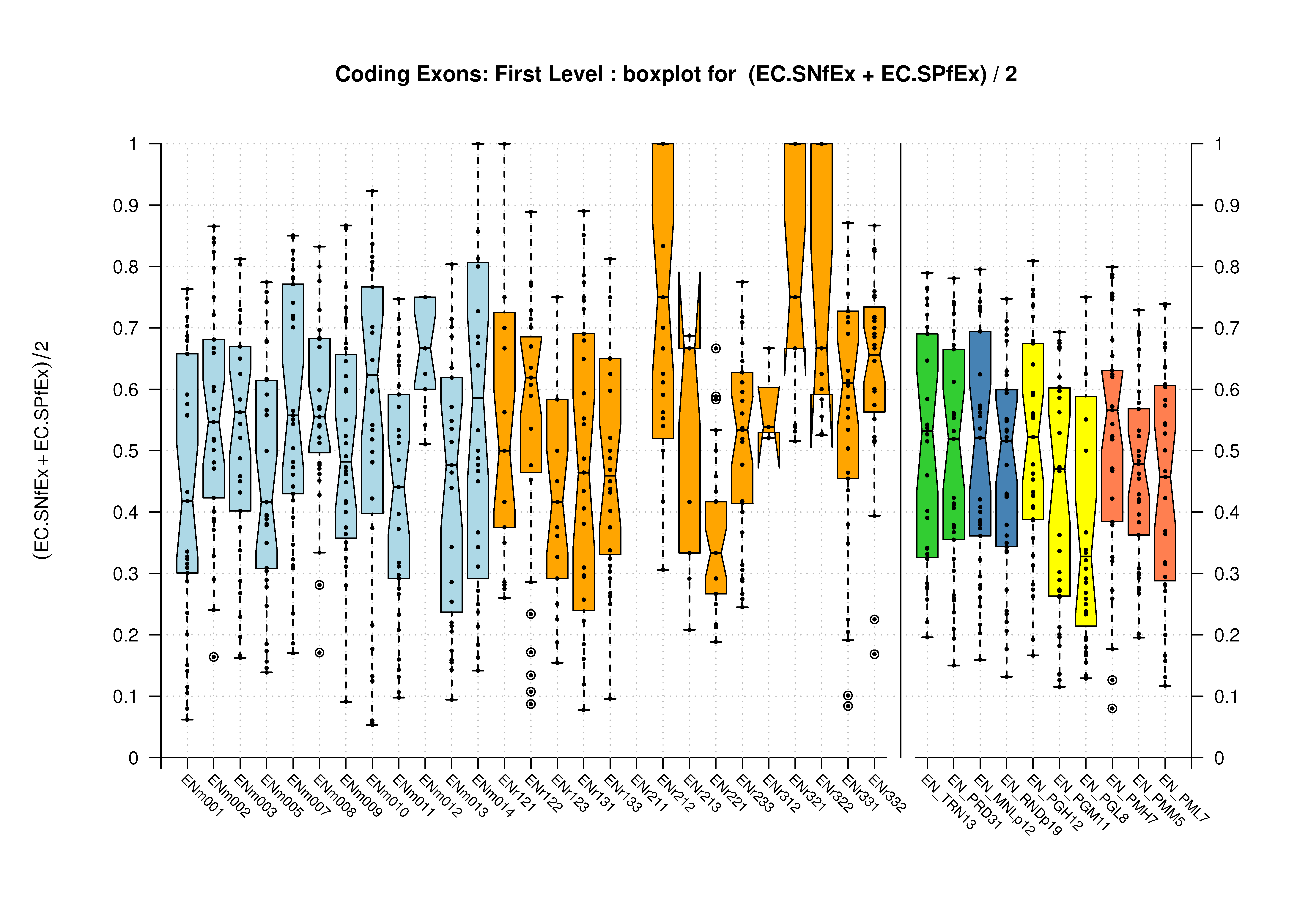 [PS][PDF][PNG] |
 [PS][PDF][PNG] |
|
| Internal Exon | 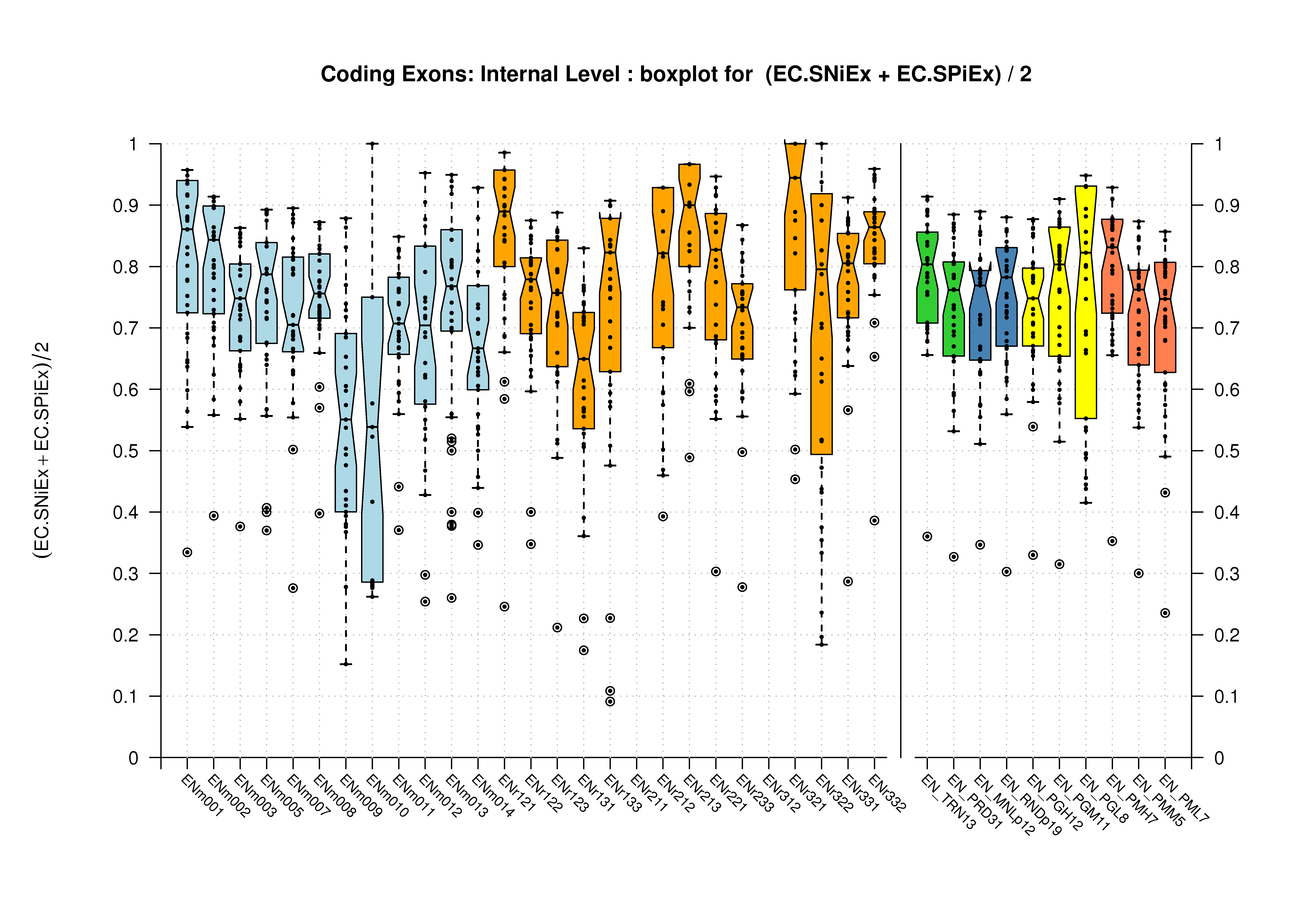 [PS][PDF][PNG] |
 [PS][PDF][PNG] |
|
| Terminal Exon | 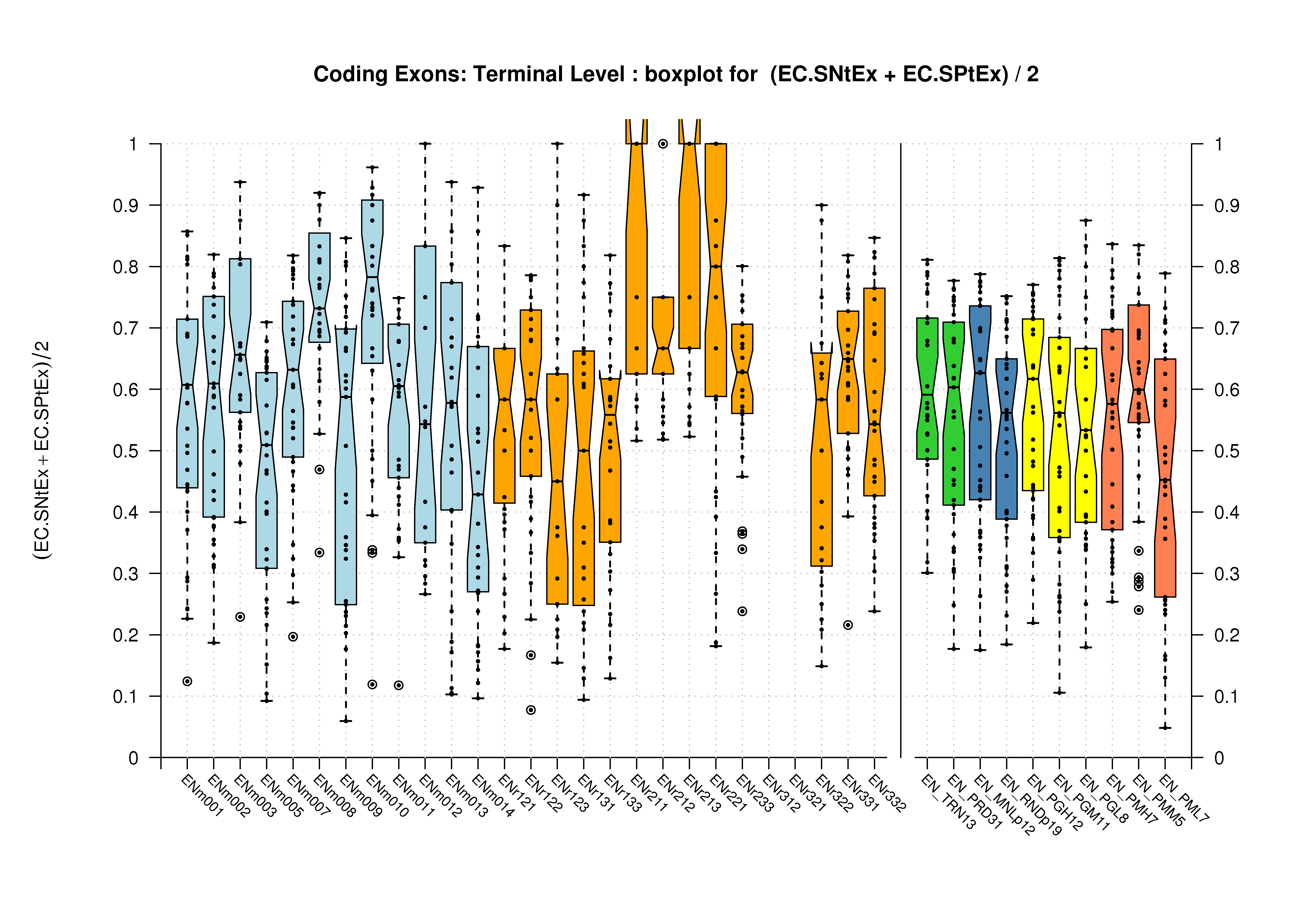 [PS][PDF][PNG] |
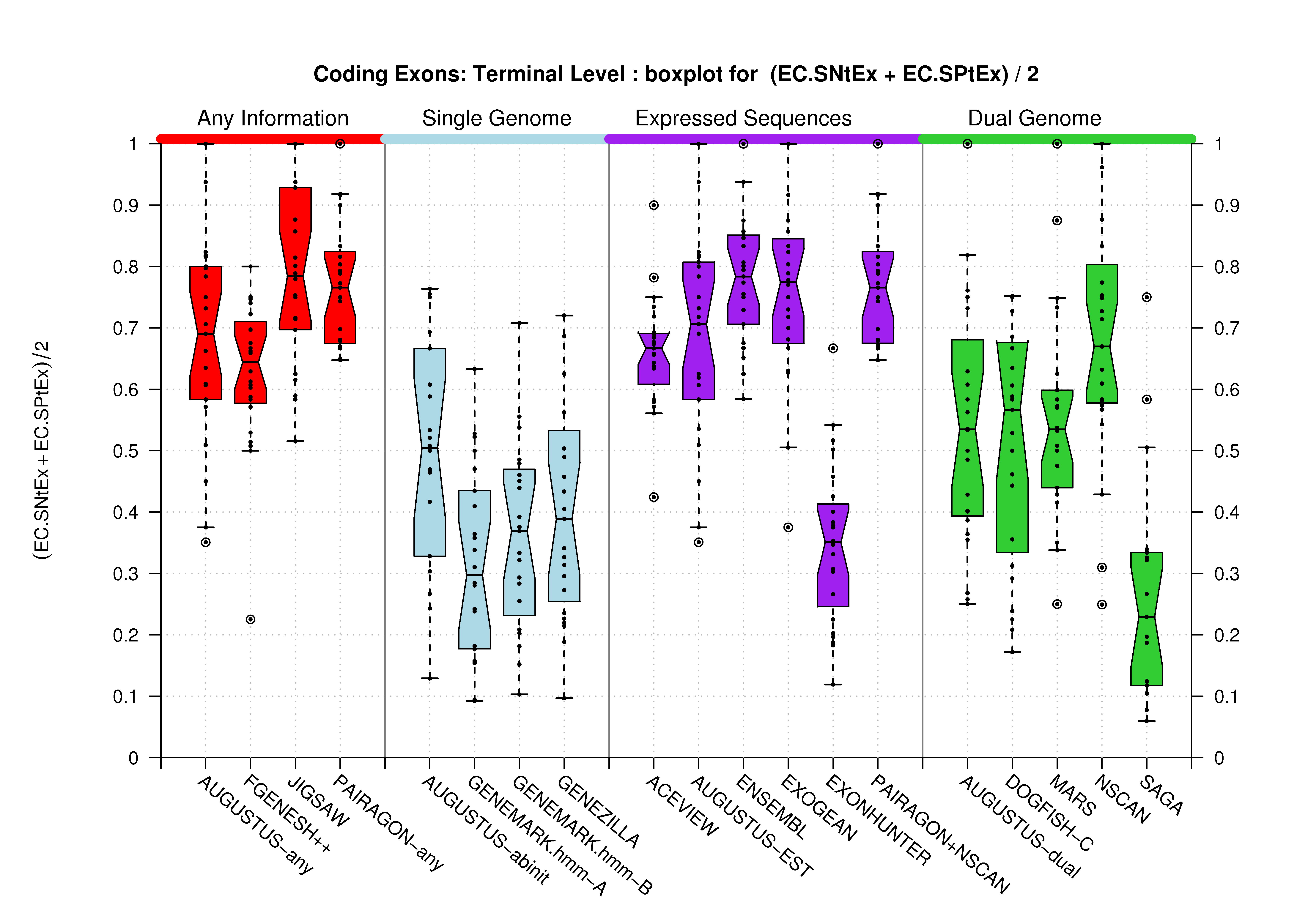 [PS][PDF][PNG] |
|
| Single Exon |  [PS][PDF][PNG] |
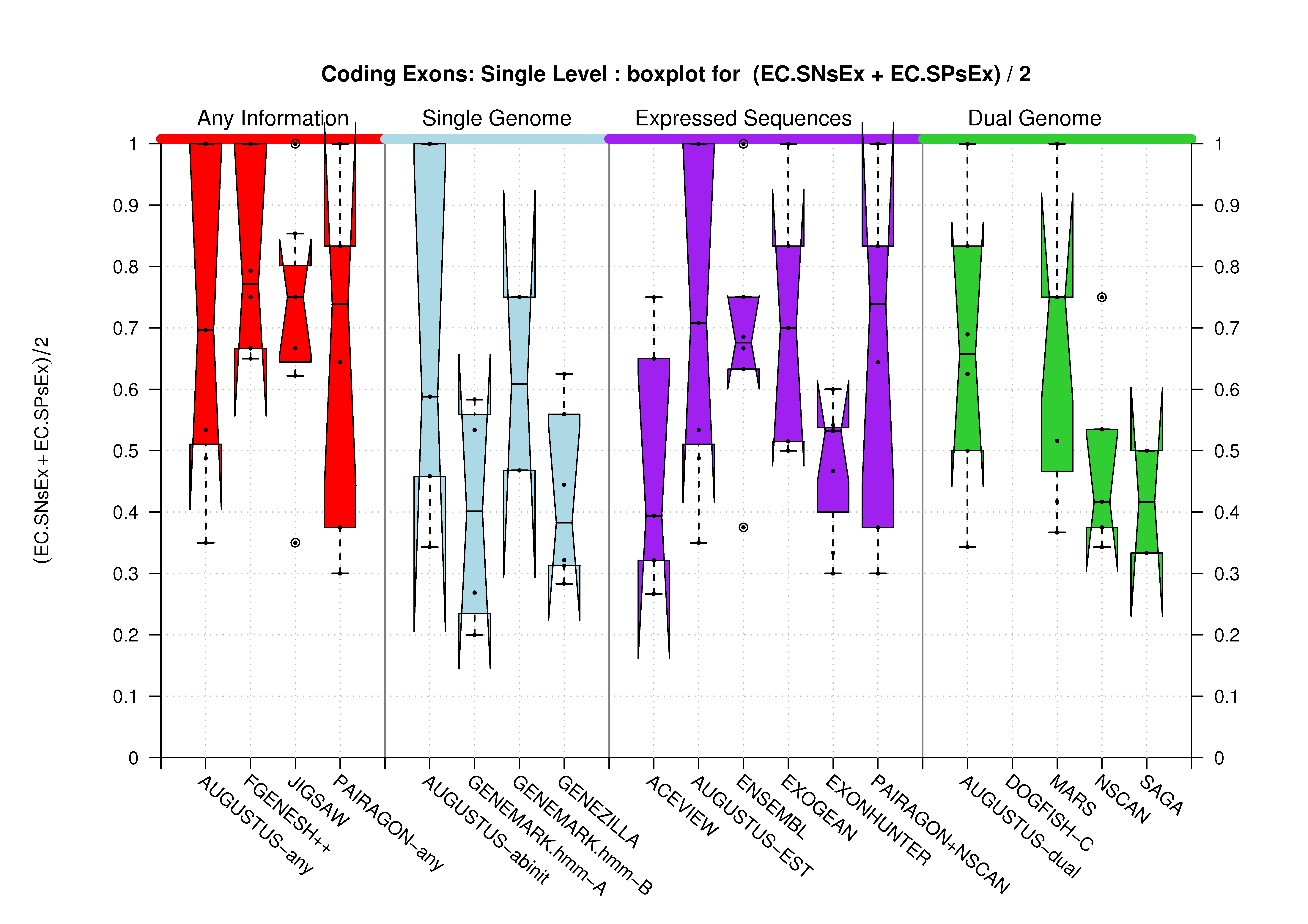 [PS][PDF][PNG] |
|
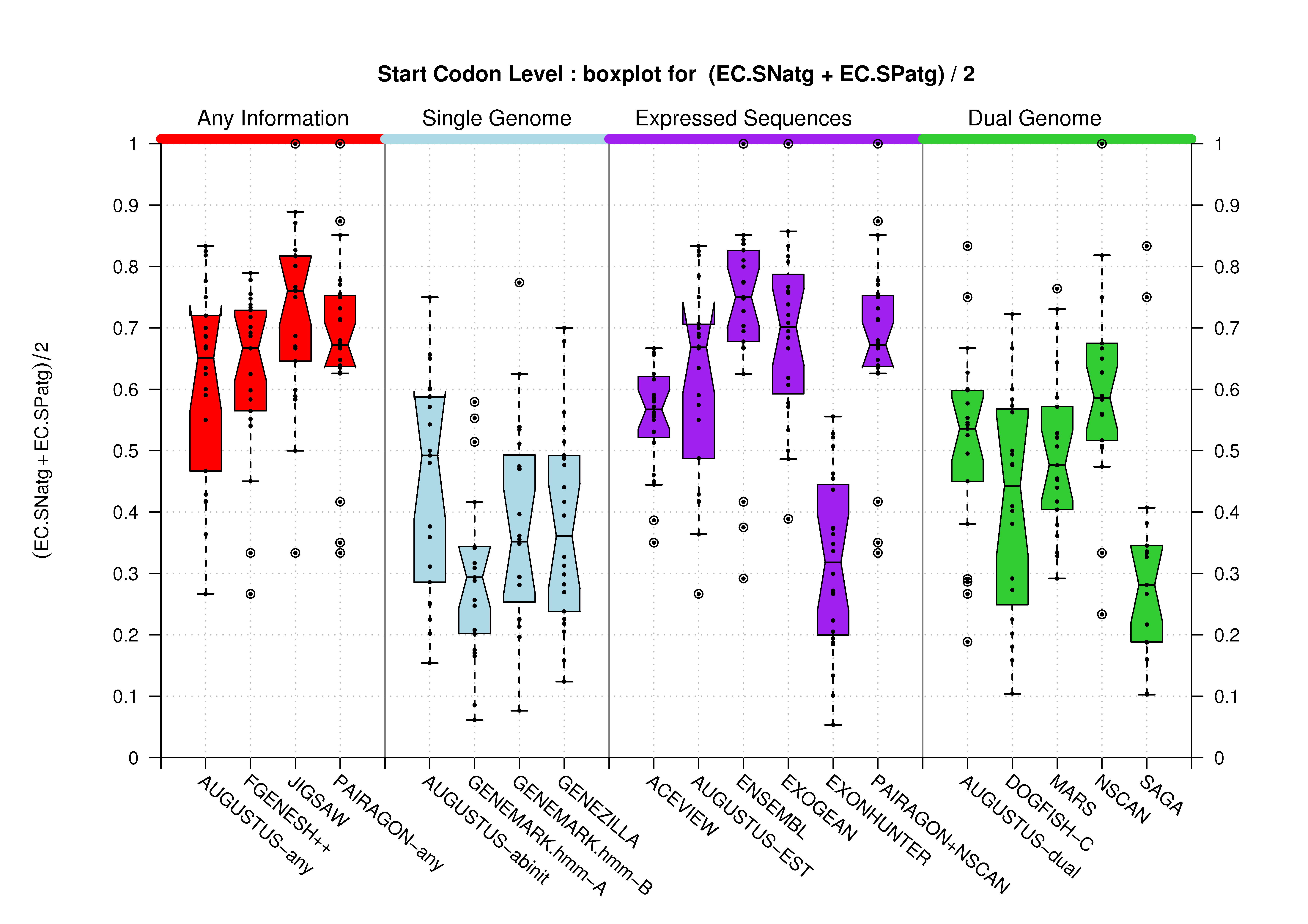
| Start Codon | 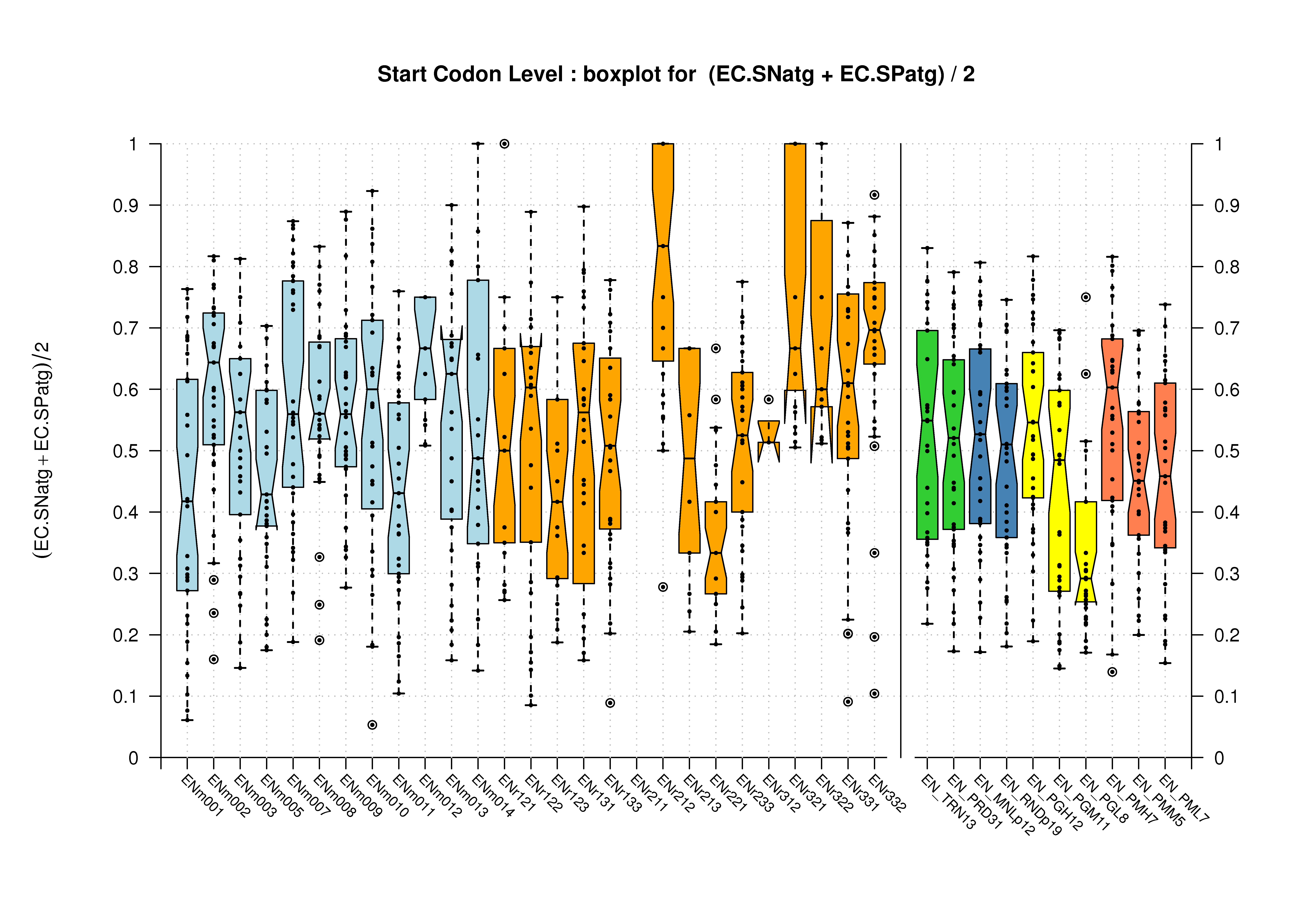 [PS][PDF][PNG] |
 [PS][PDF][PNG] |
|
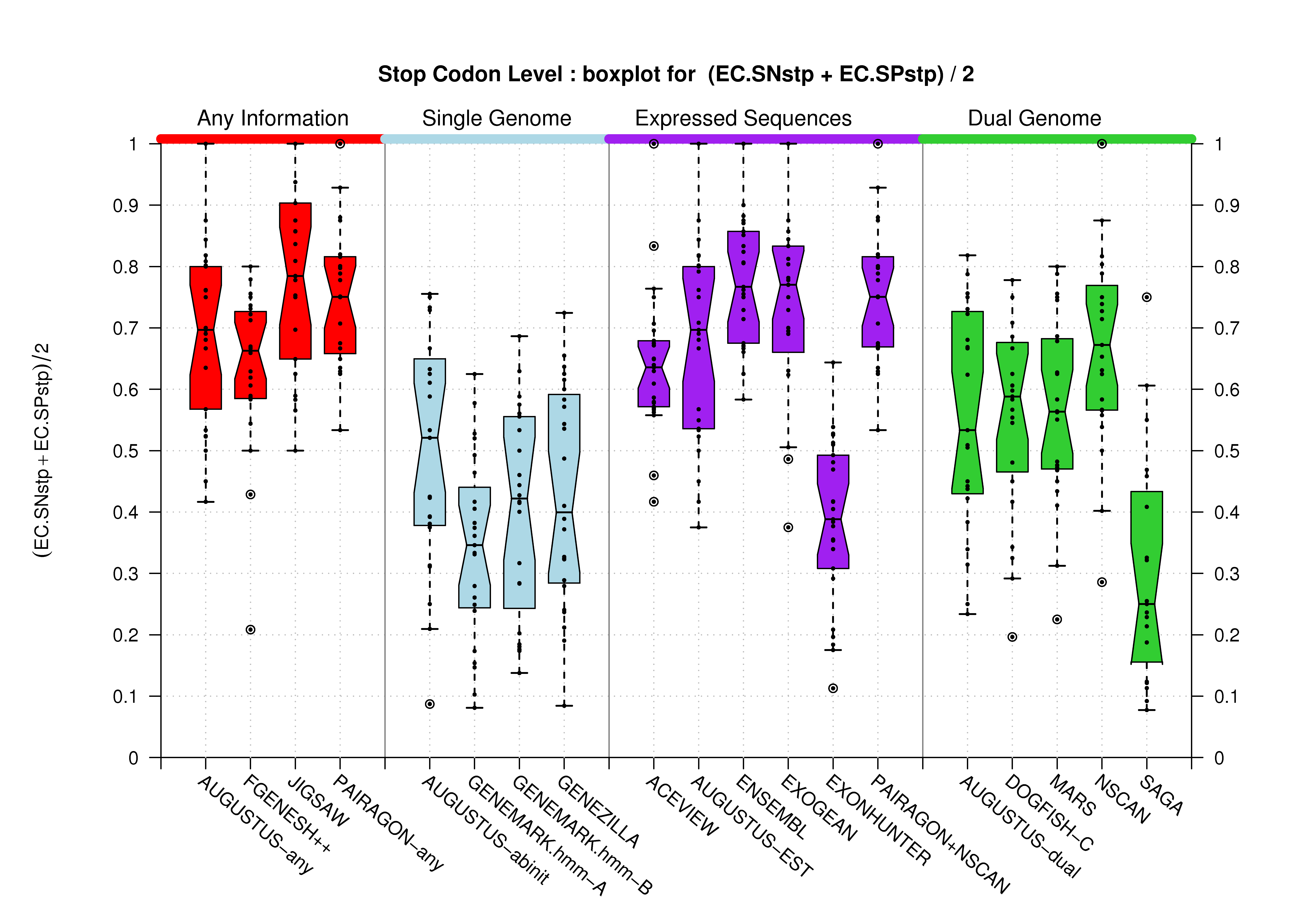
| Stop Codon | 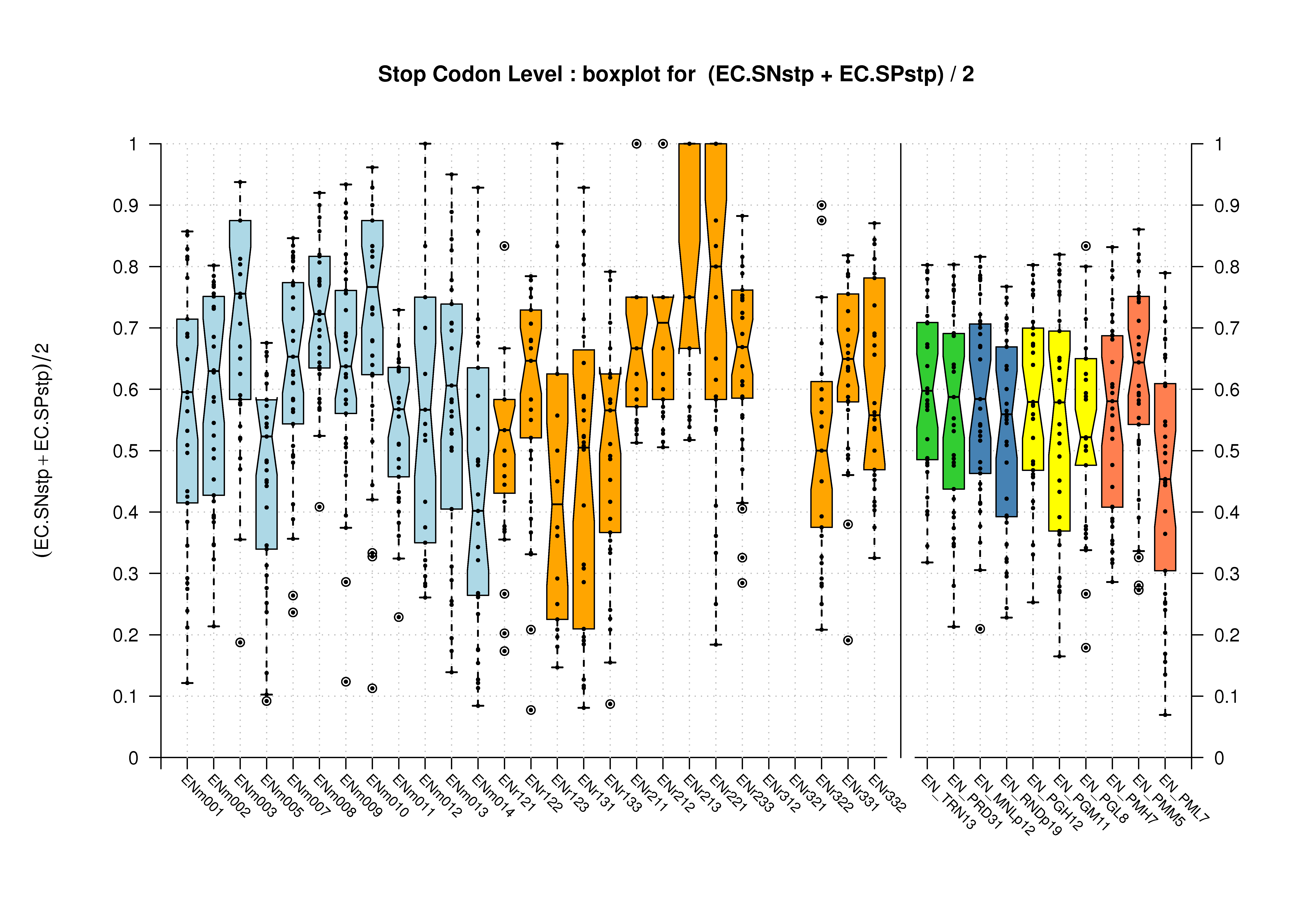 [PS][PDF][PNG] |
 [PS][PDF][PNG] |
|
Sample sizes are smaller for the Single exons case. This is reflected in the shape of the boxplots. On the other hand, from the above figures one can see that Internal exons is the class having better results than First or Terminal exons.
Exon Level
| Feature | Havana Coding Genes Dataset | Havana Genes Dataset | |
|---|---|---|---|
| All Exons | 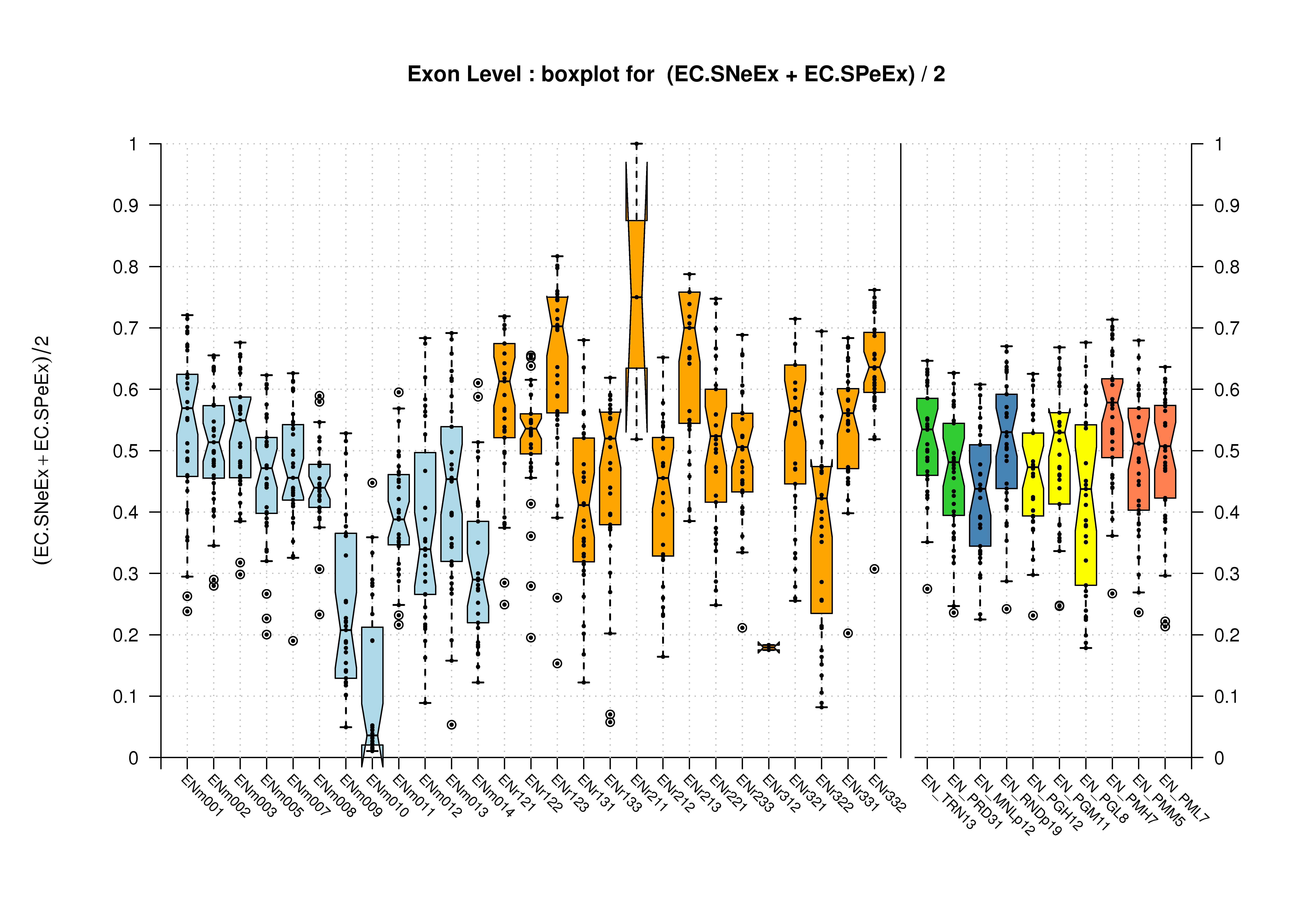 [PS][PDF][PNG] |
 [PS][PDF][PNG] |
 [PS][PDF][PNG] |
| All Introns | 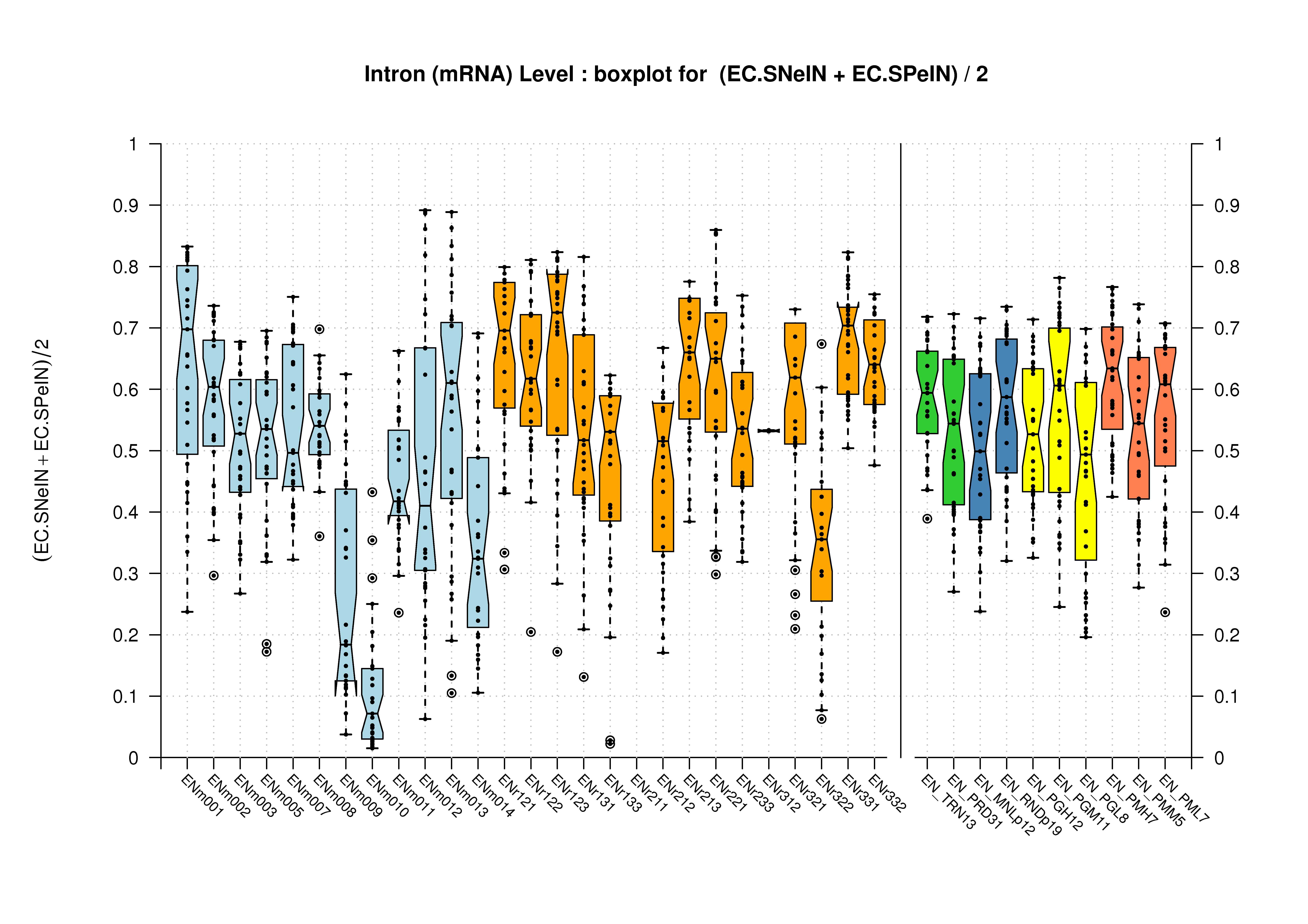 [PS][PDF][PNG] |
 [PS][PDF][PNG] |
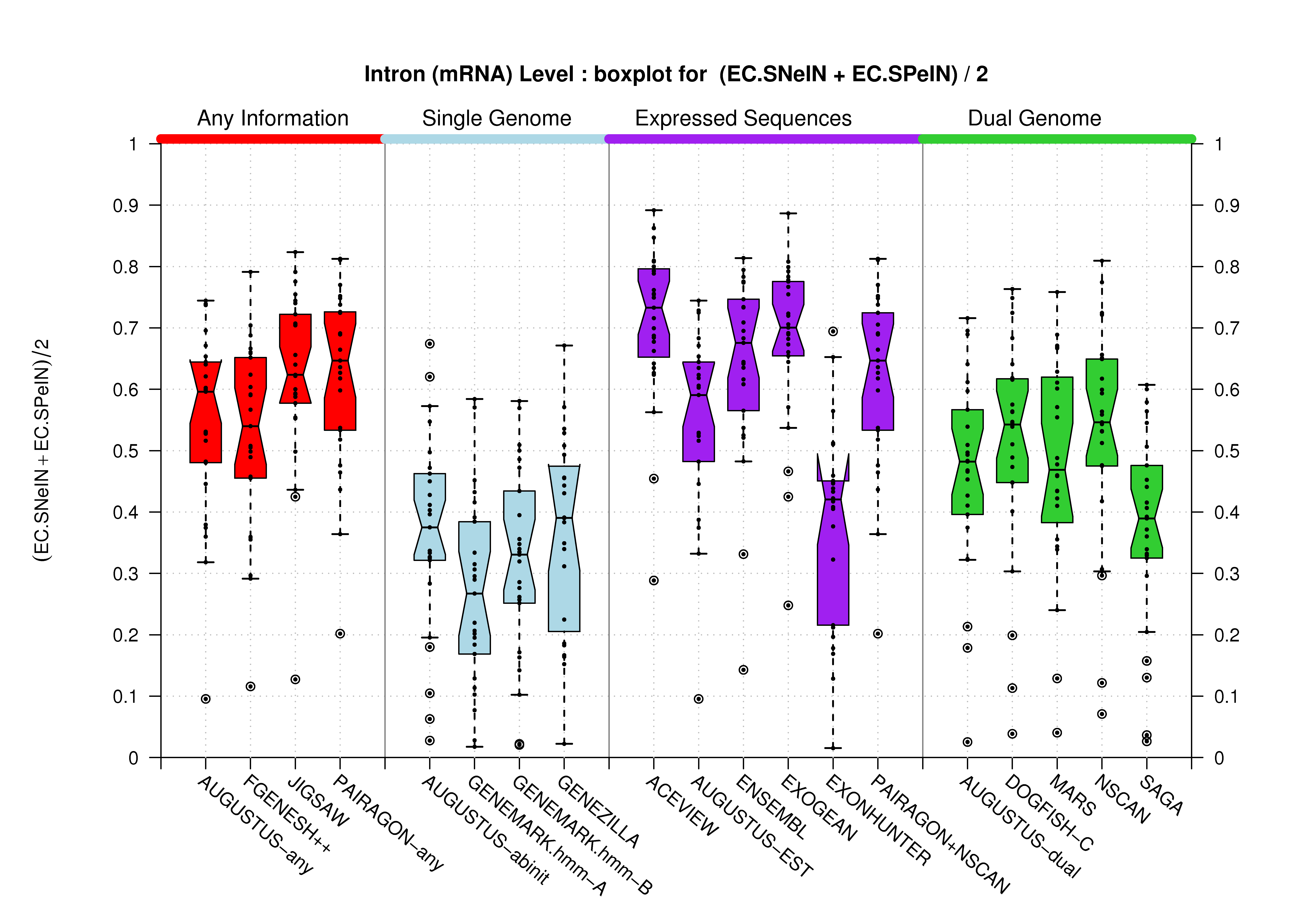 [PS][PDF][PNG] |
| Transcription Start Site (TSS) |
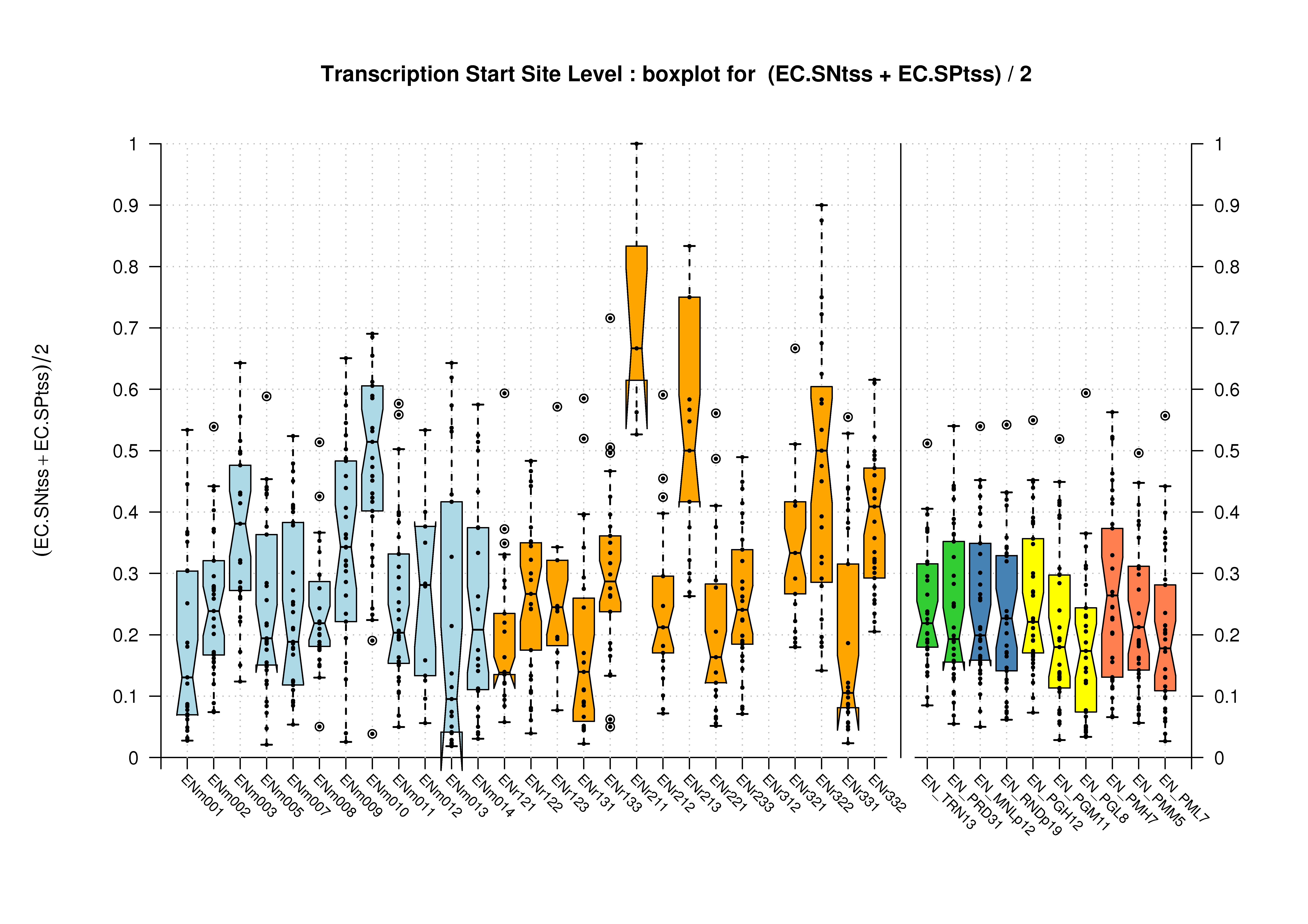 [PS][PDF][PNG] |
 [PS][PDF][PNG] |
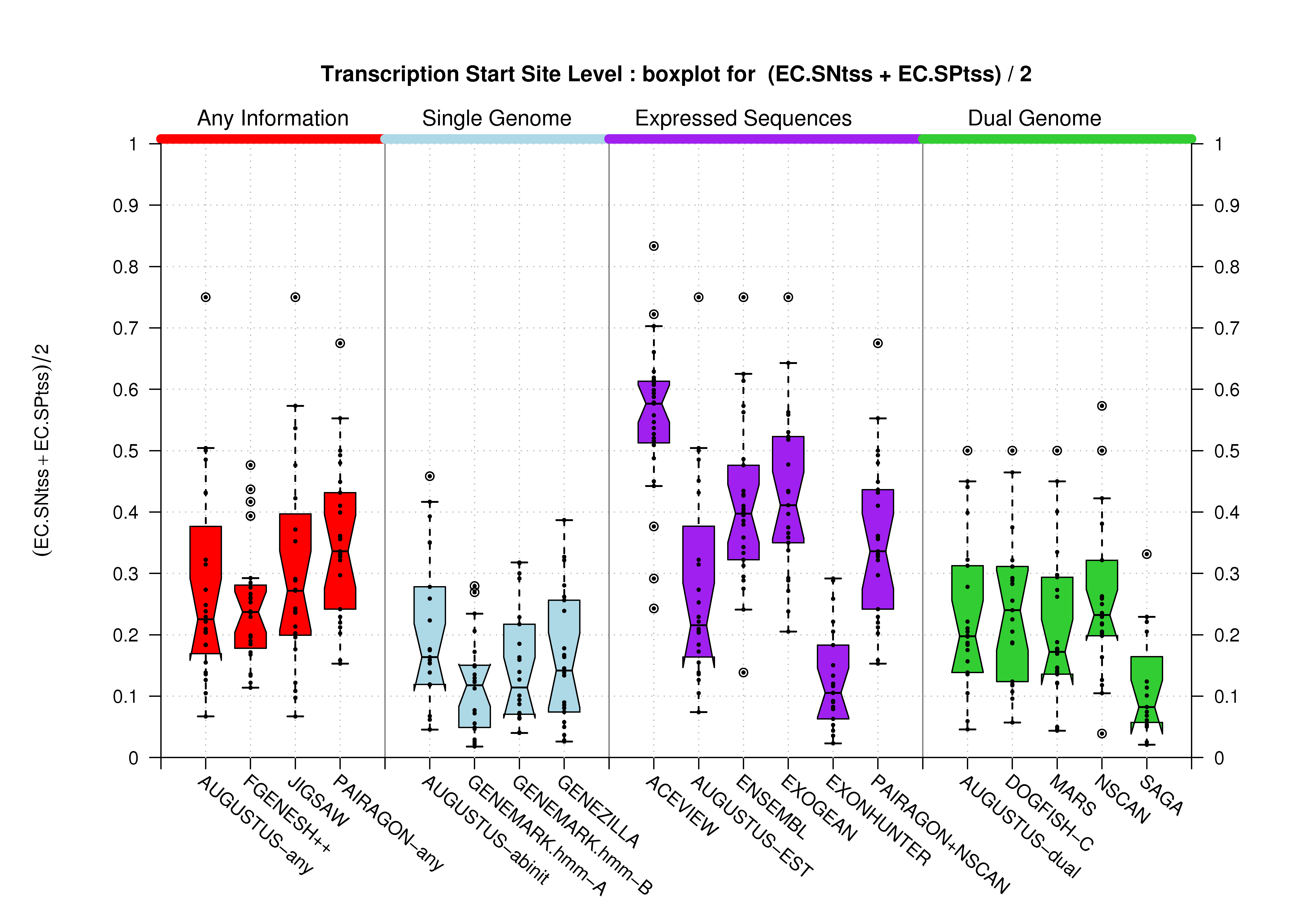 [PS][PDF][PNG] |
| Transcription End Site (TSS) |
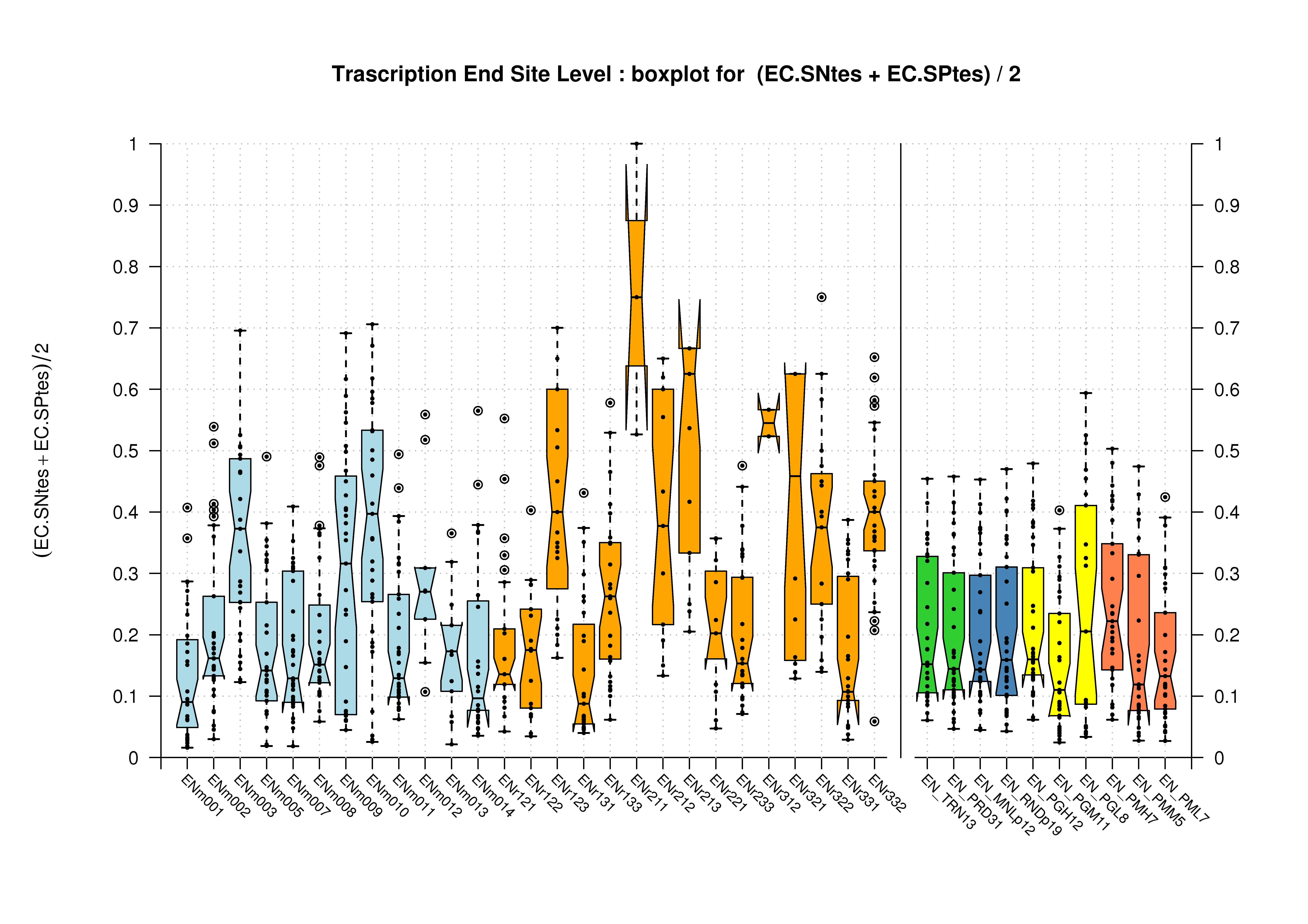 [PS][PDF][PNG] |
 [PS][PDF][PNG] |
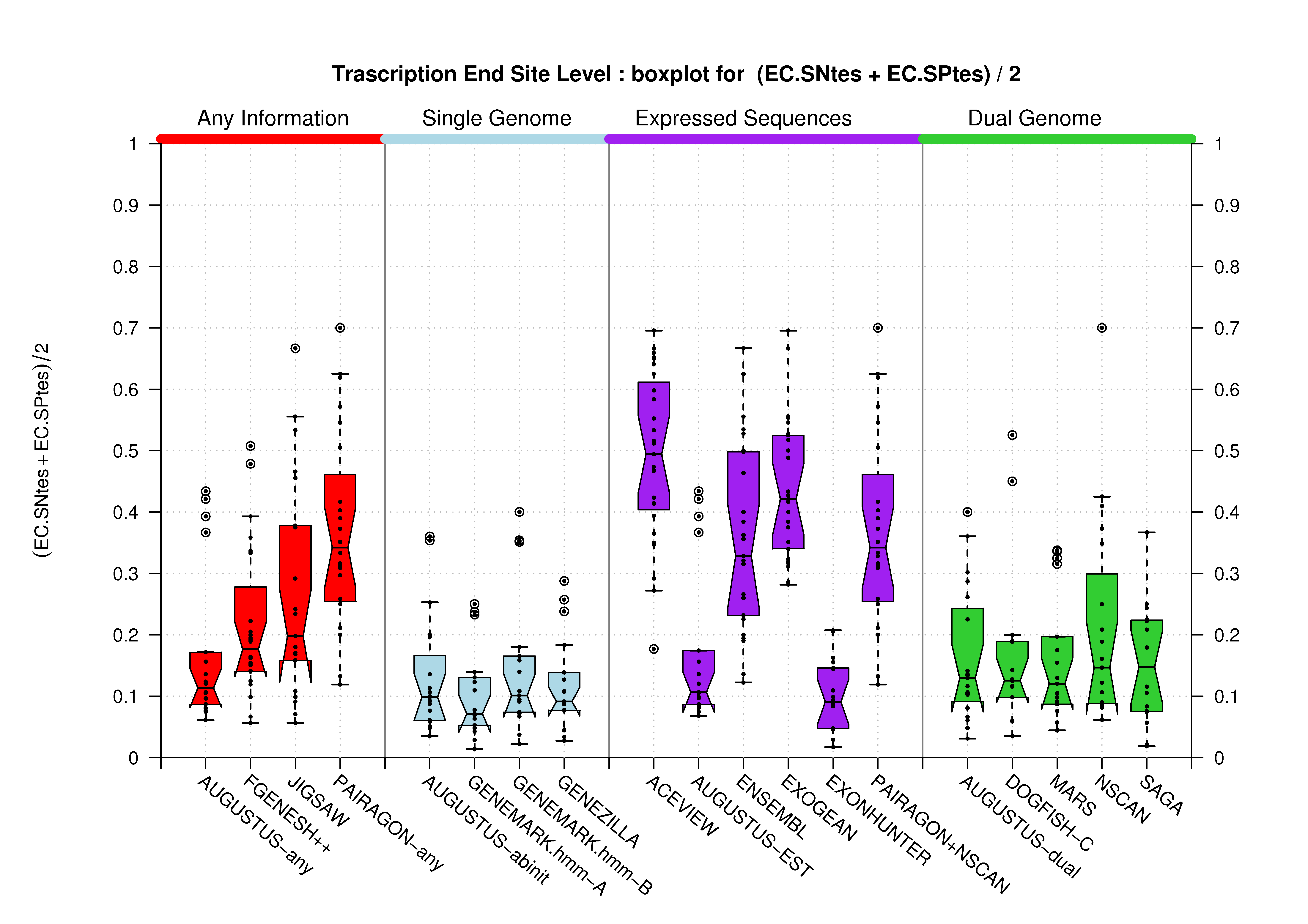 [PS][PDF][PNG] |
Splice Sites
| Feature | Havana Coding Genes Dataset | Havana Genes Dataset | |
|---|---|---|---|
| Donor Site (Coding Exons) |
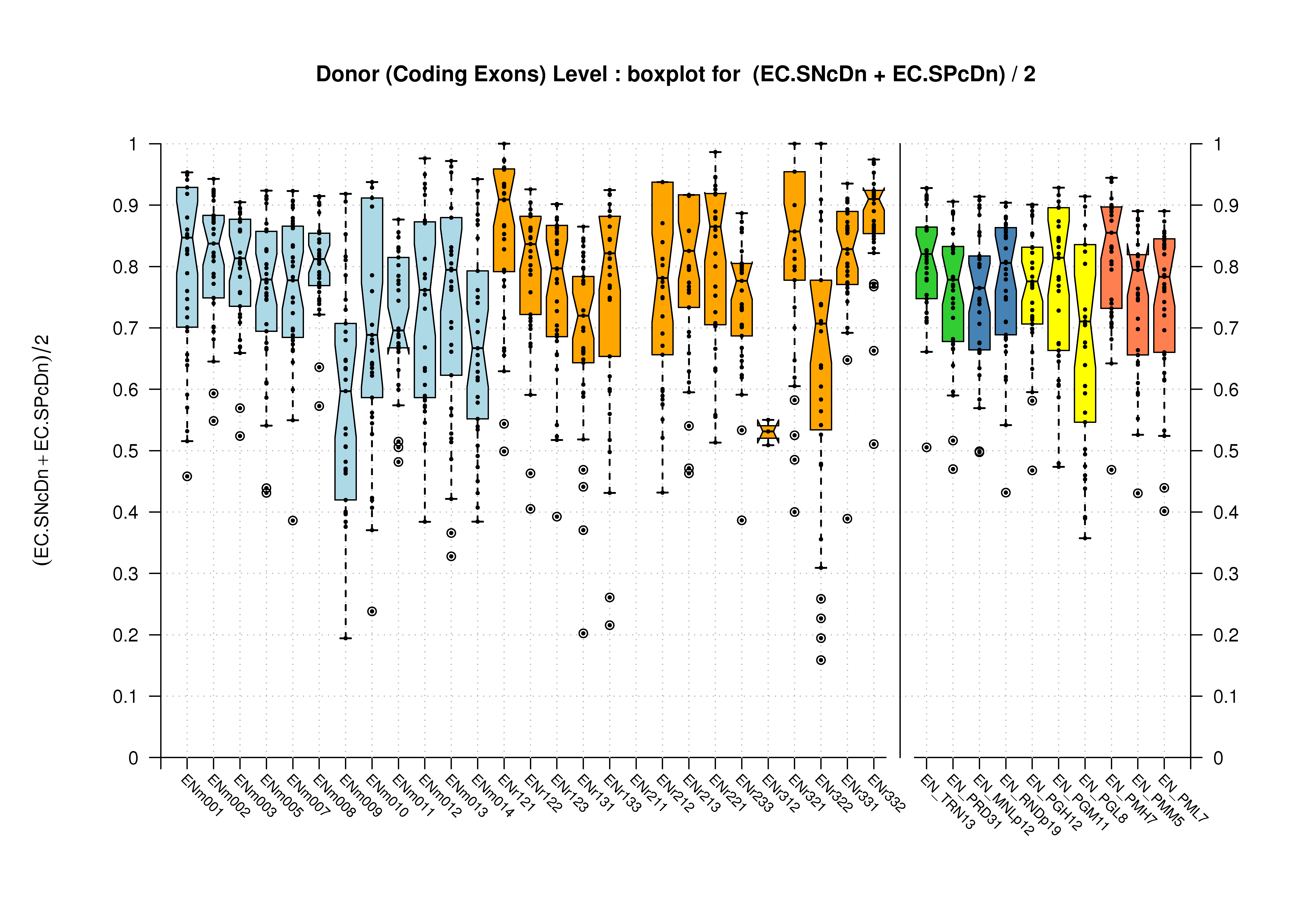 [PS][PDF][PNG] |
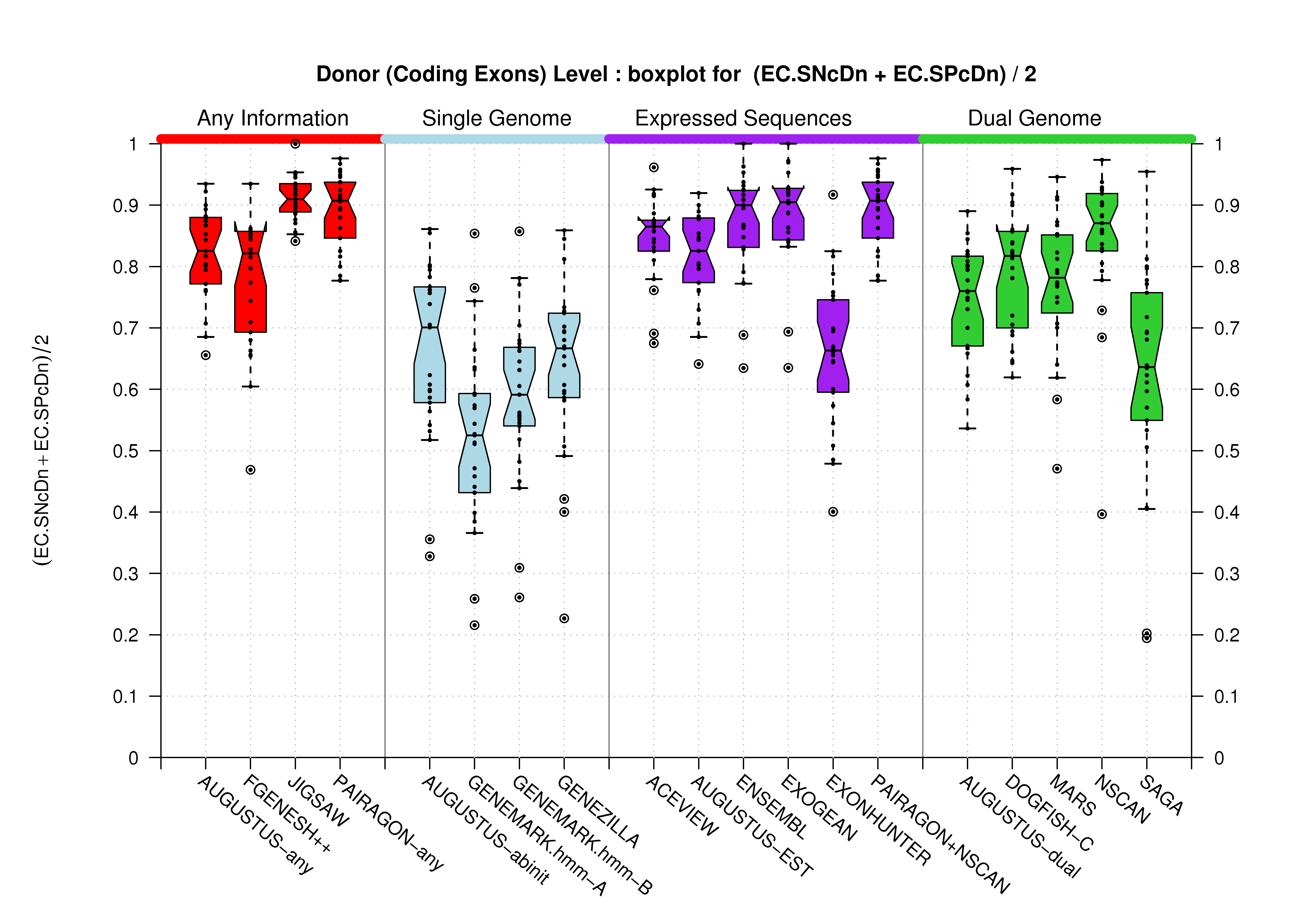 [PS][PDF][PNG] |
|
| Donor Site (All Exons) |
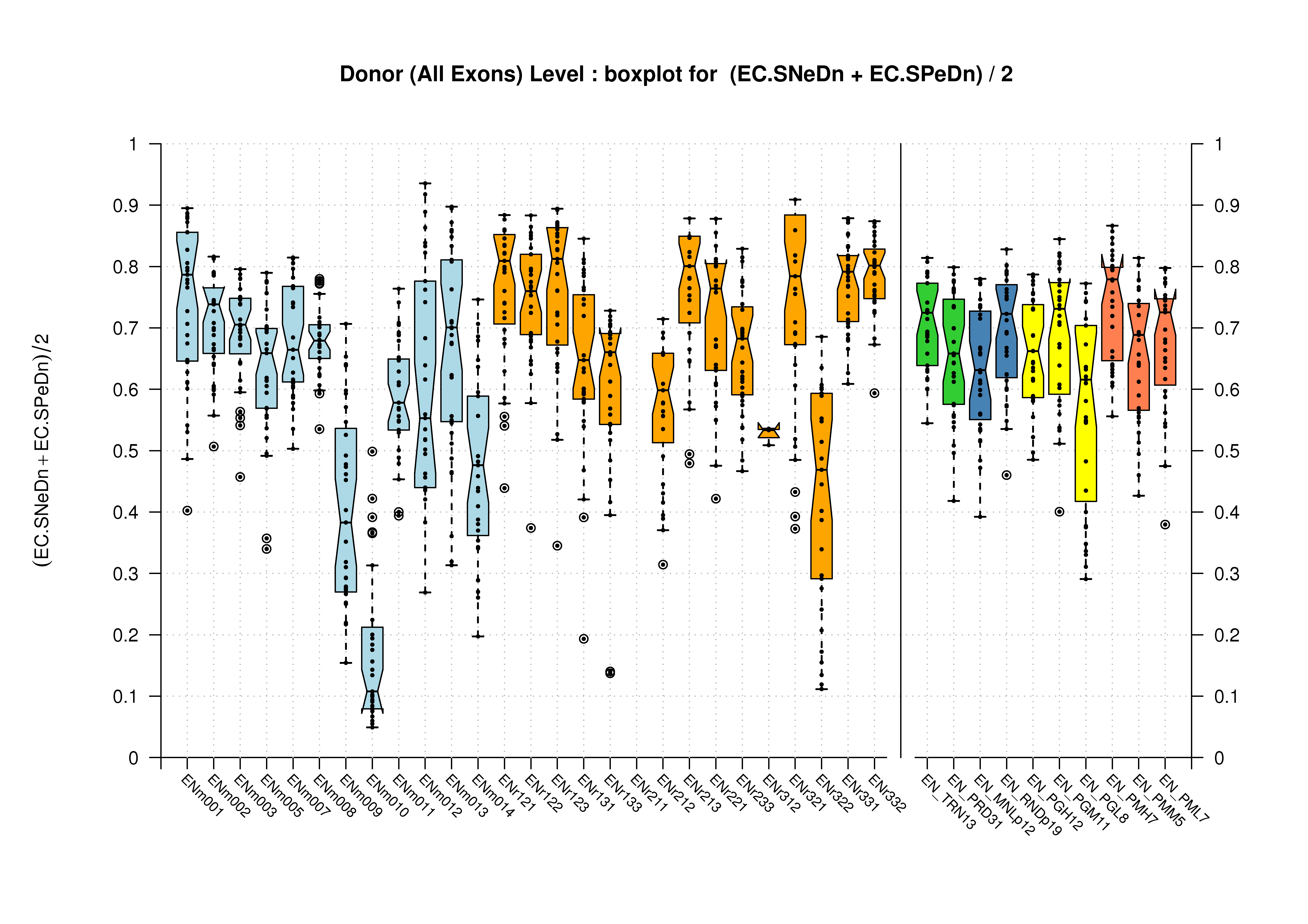 [PS][PDF][PNG] |
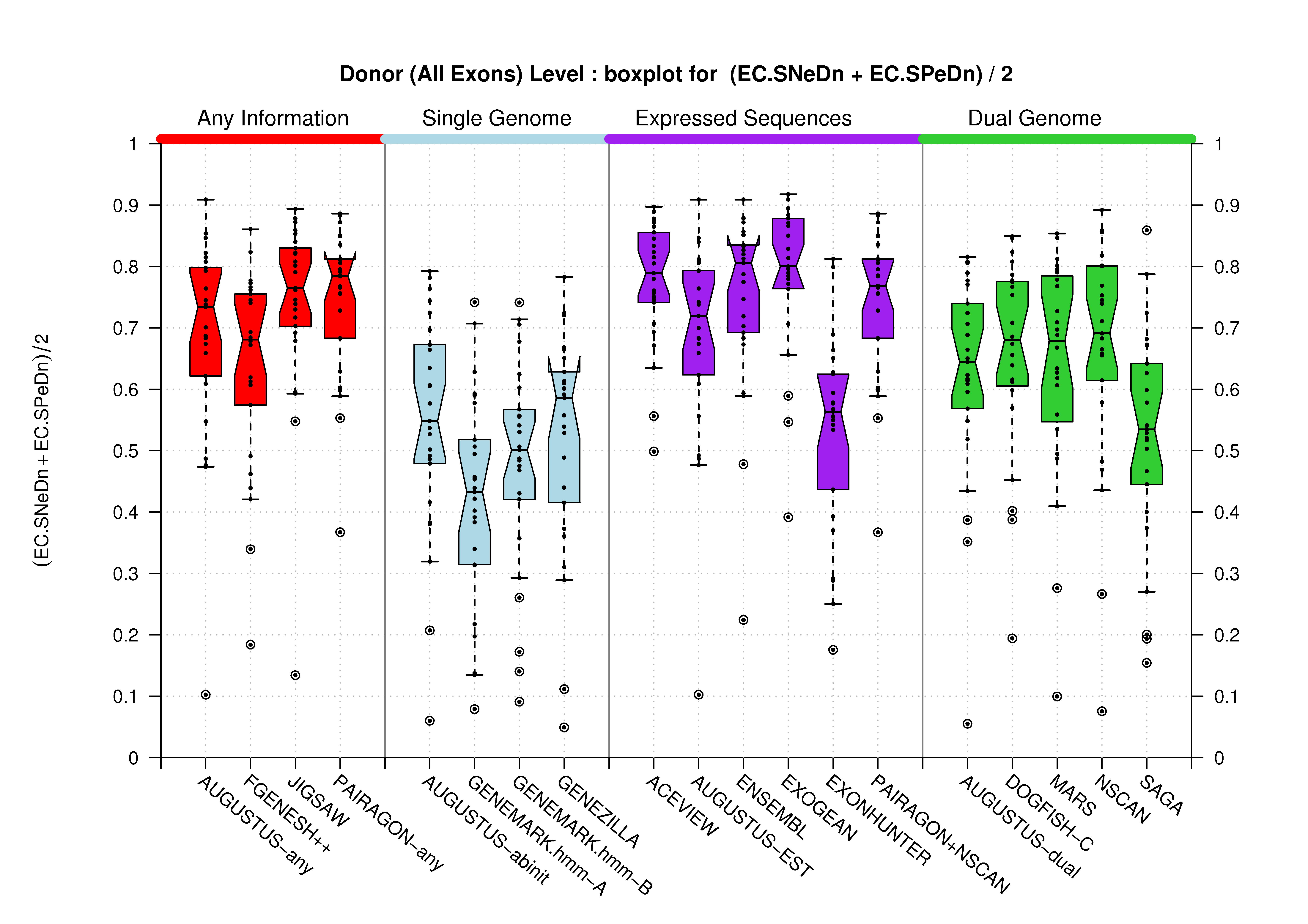 [PS][PDF][PNG] |
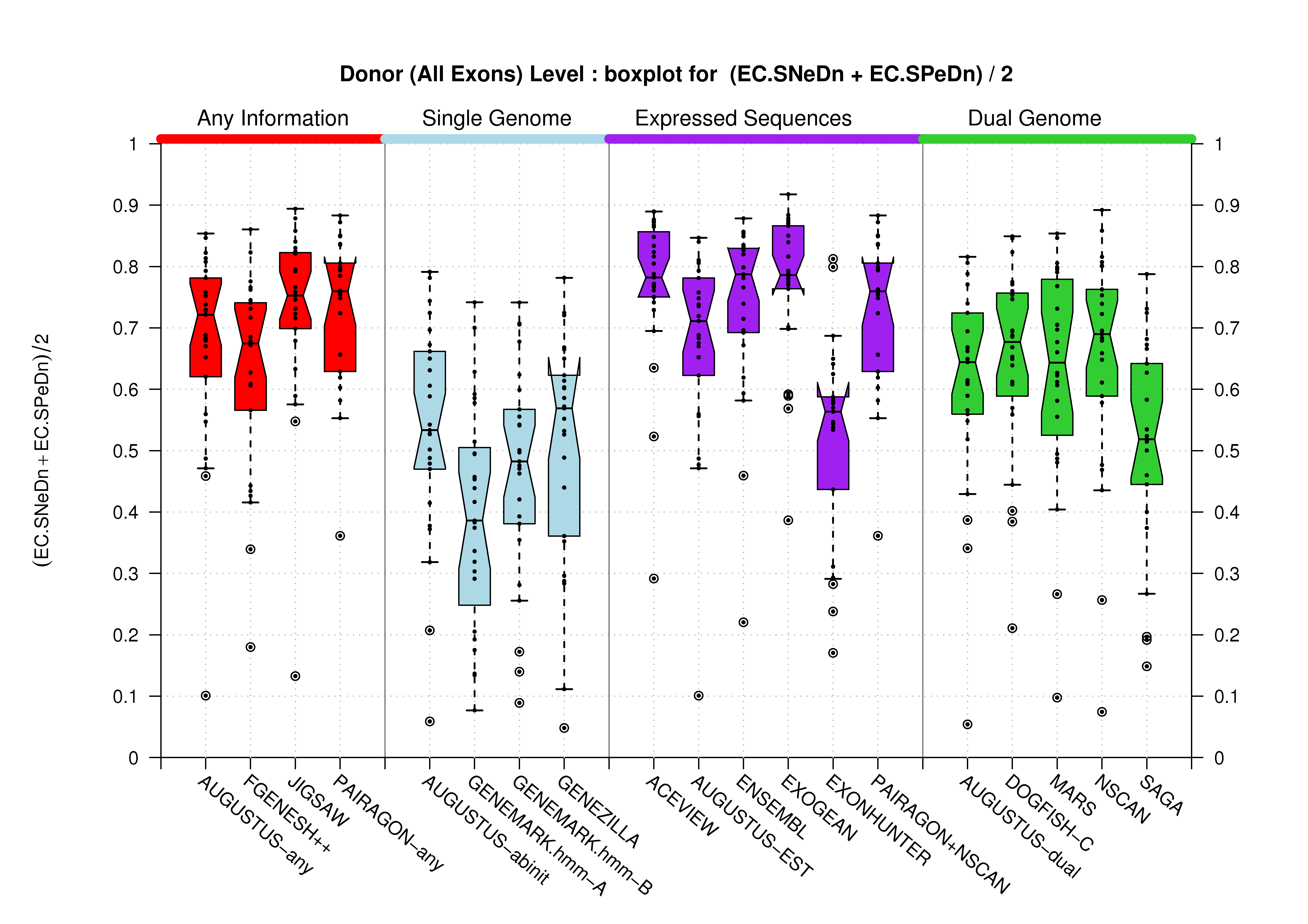 [PS][PDF][PNG] |
| Acceptor Site (Coding Exons) |
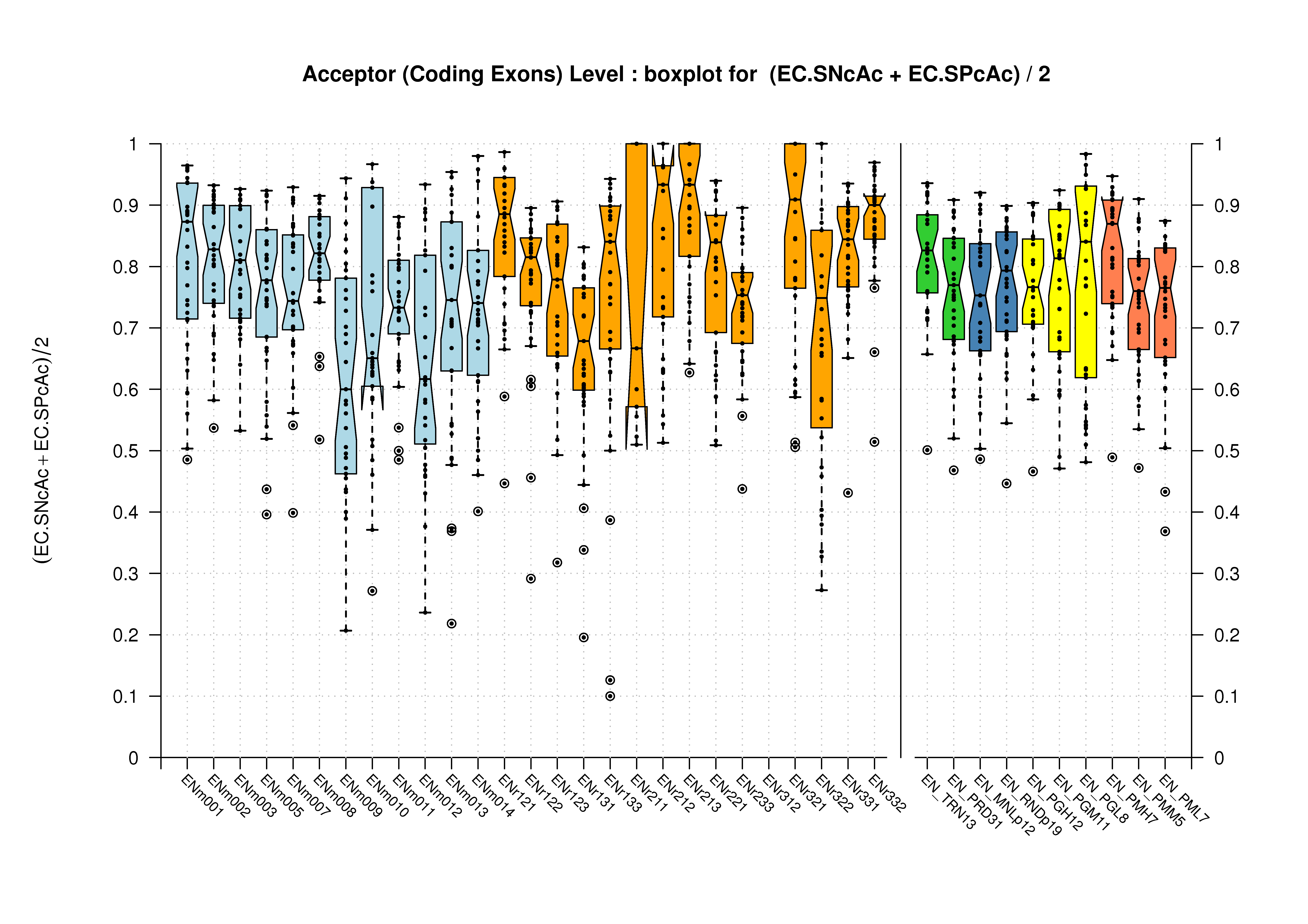 [PS][PDF][PNG] |
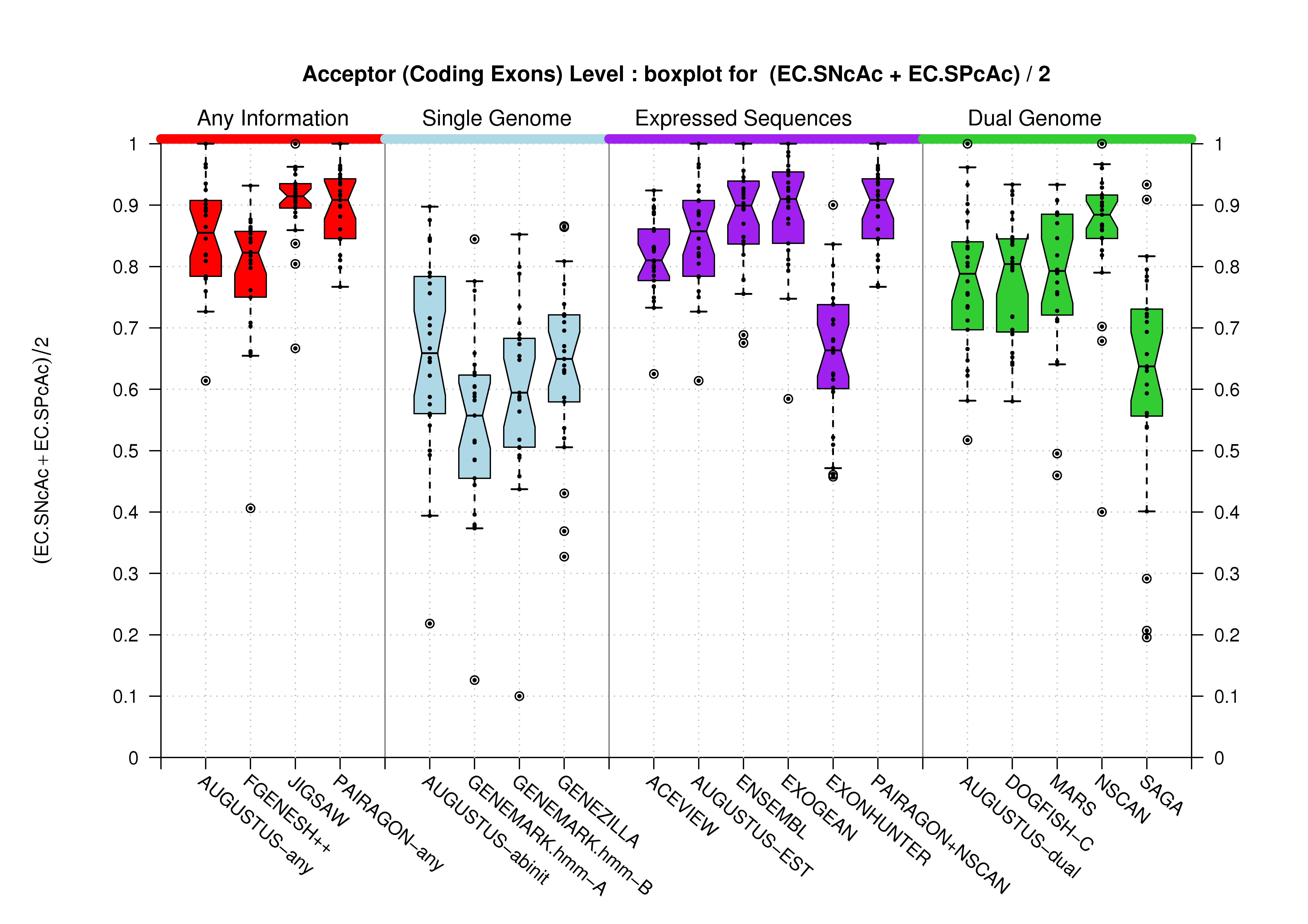 [PS][PDF][PNG] |
|
| Acceptor Site (All Exons) |
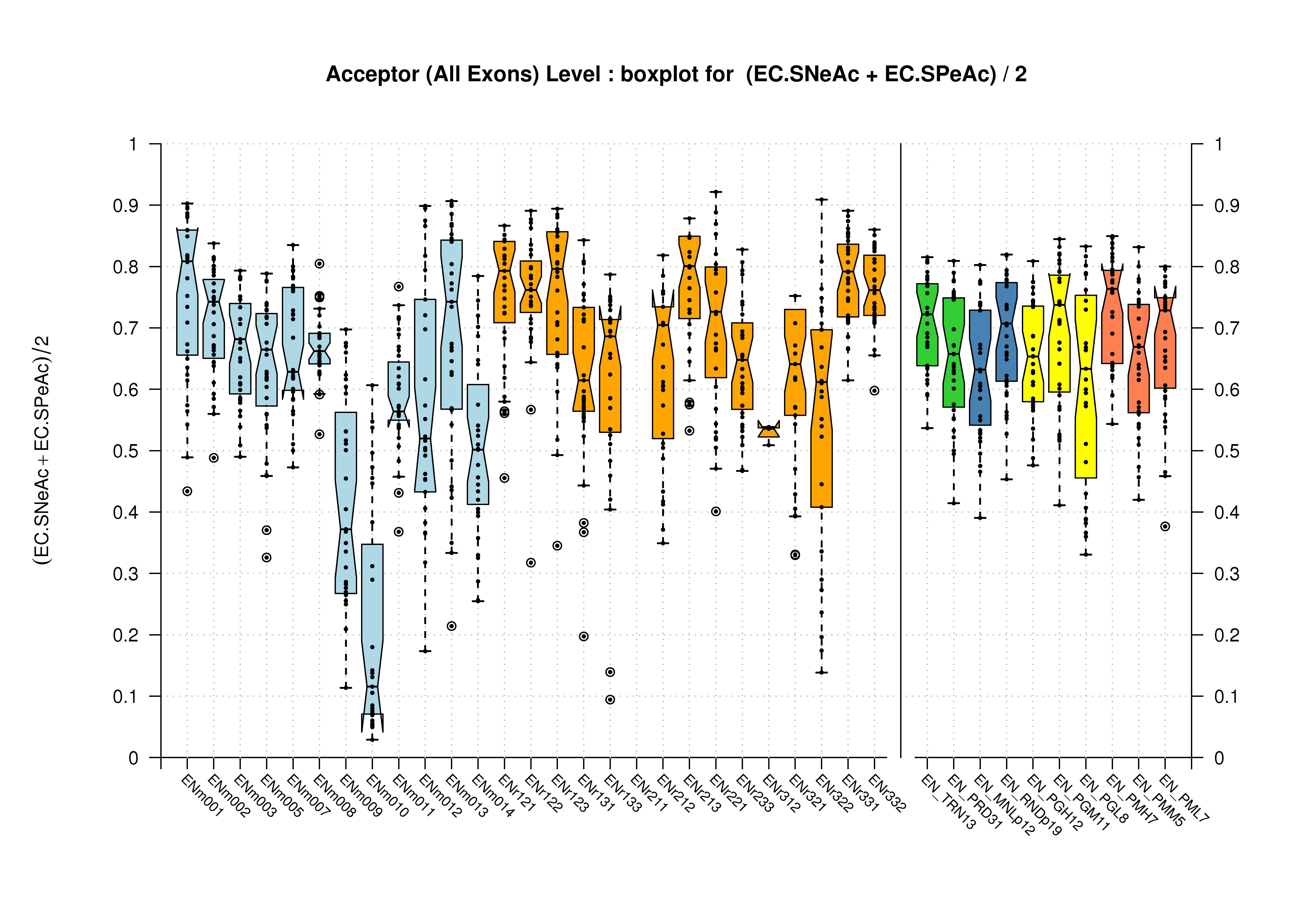 [PS][PDF][PNG] |
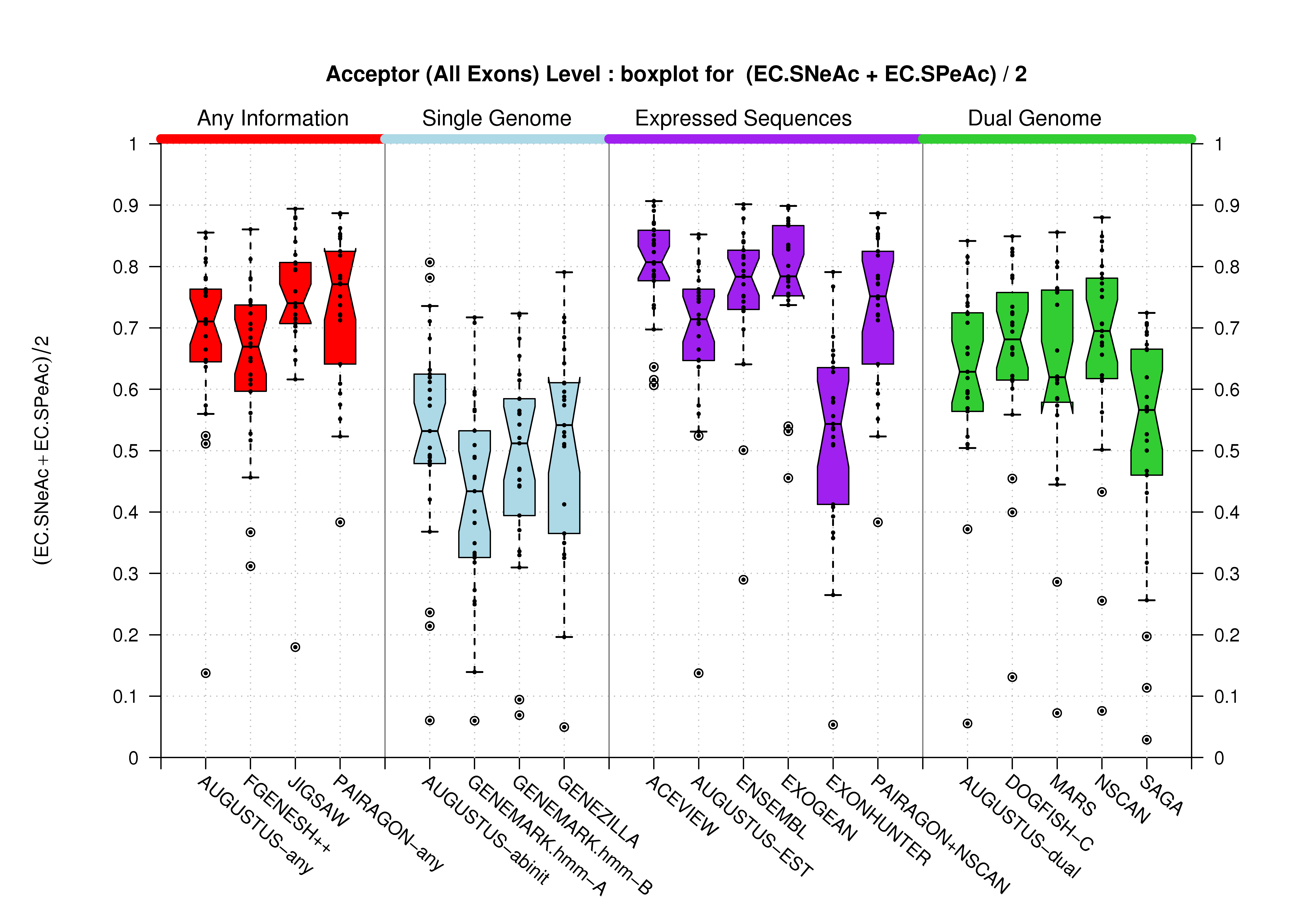 [PS][PDF][PNG] |
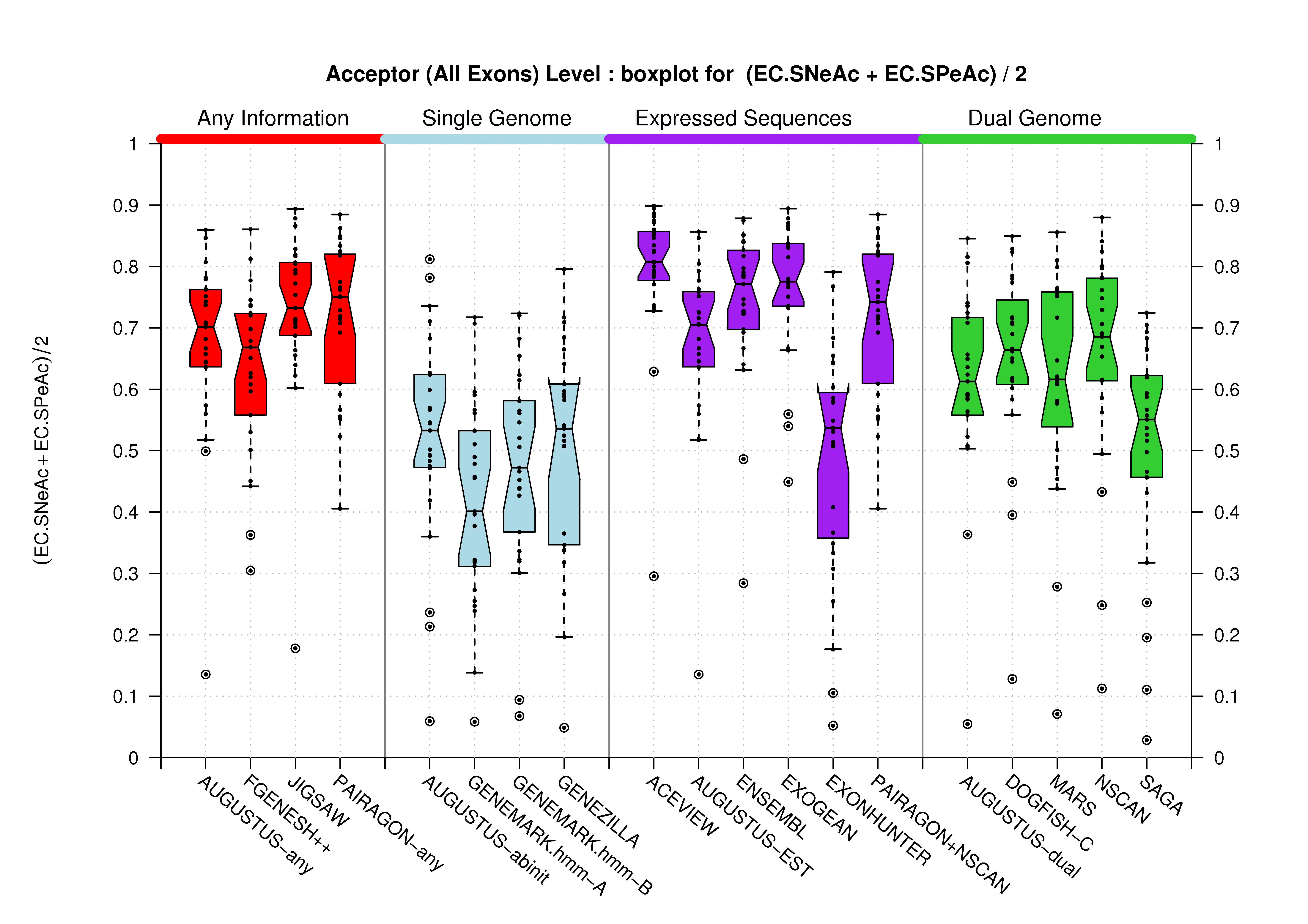 [PS][PDF][PNG] |
Gene/Transcript Level
| Feature | Havana Coding Genes Dataset | ||
|---|---|---|---|
| Transcript | 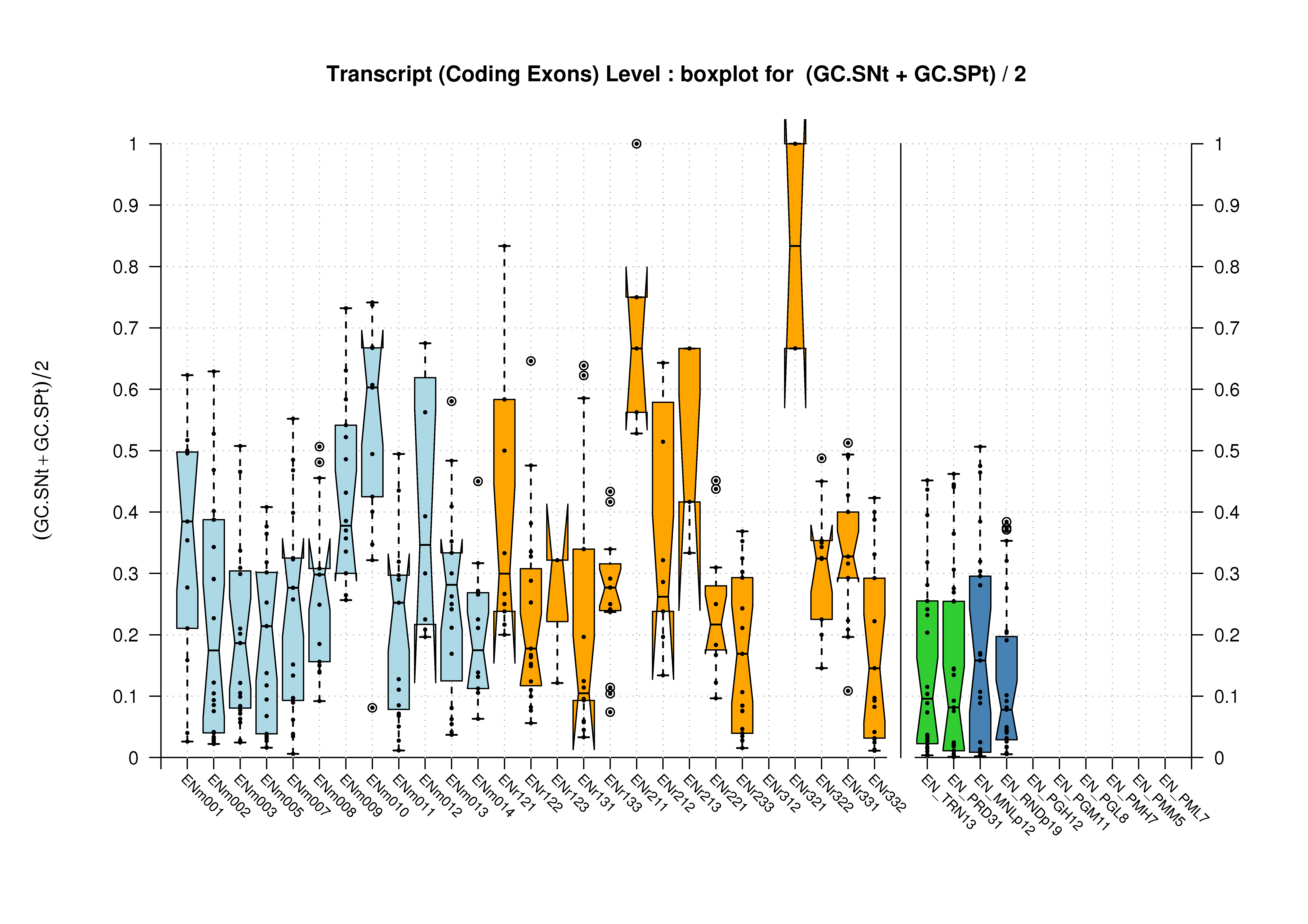 [PS][PDF][PNG] |
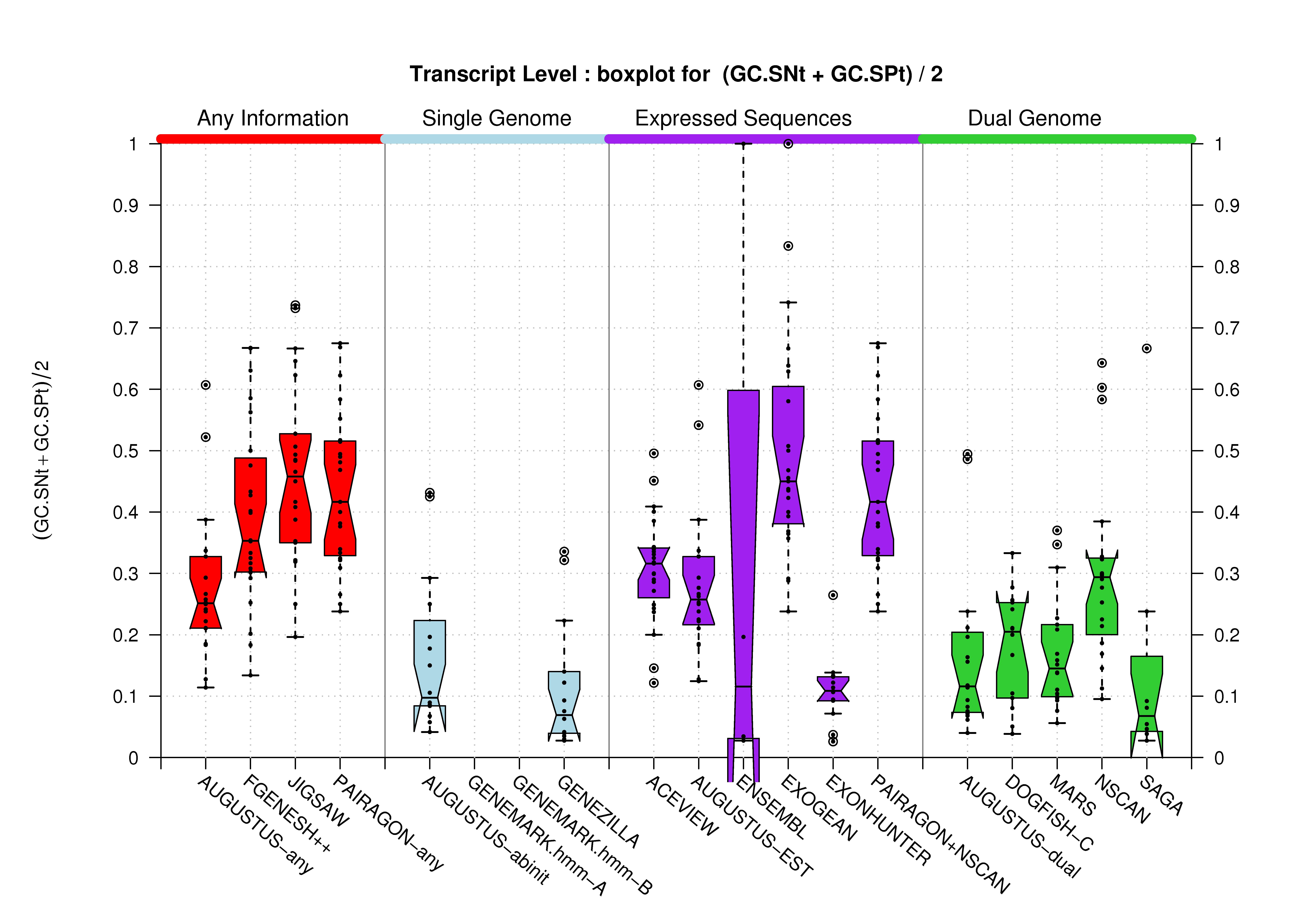 [PS][PDF][PNG] |
|
| Gene | 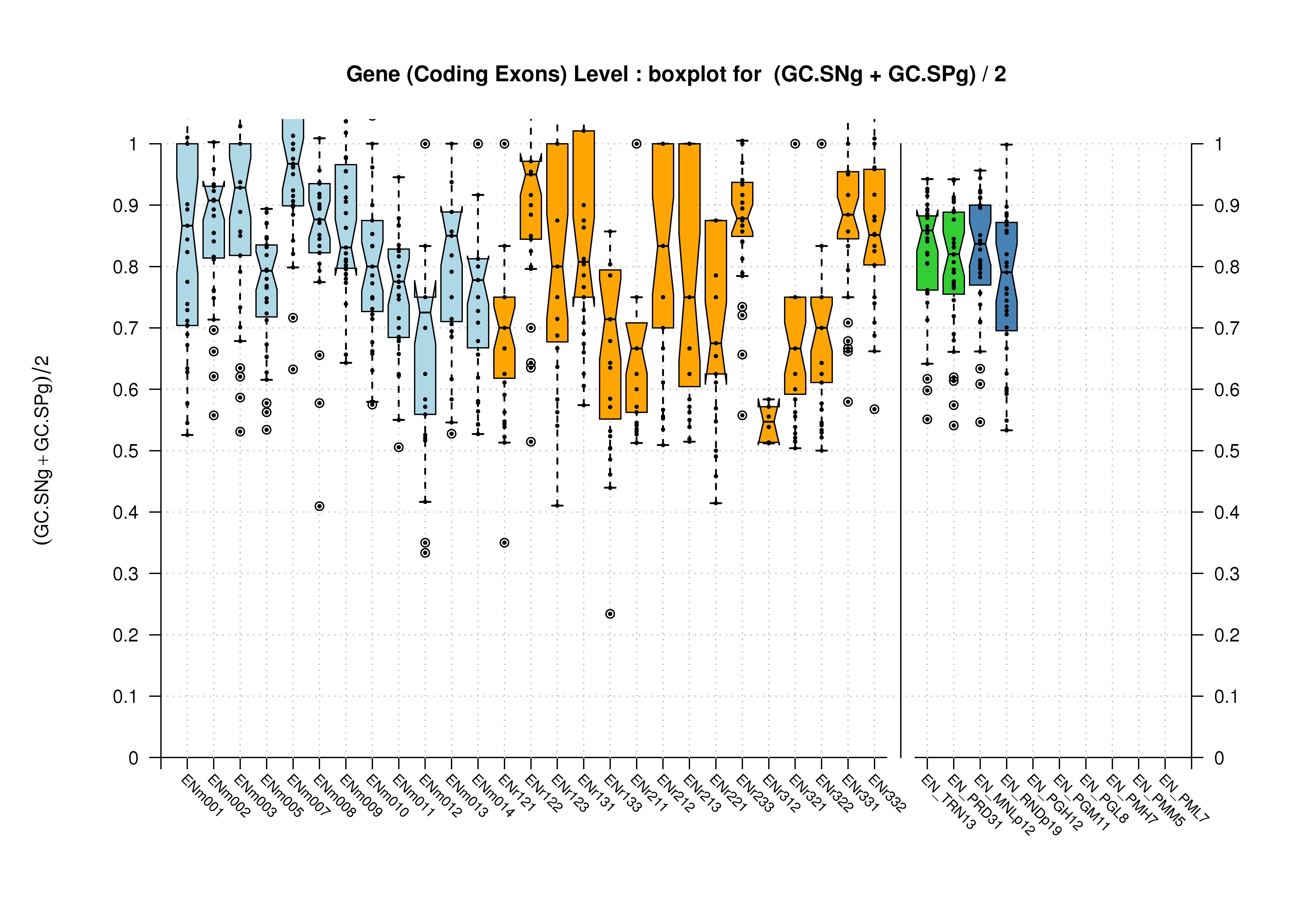 [PS][PDF][PNG] |
 [PS][PDF][PNG] |
|
We were unable to properly test all the changes made to the original Eduardo's evaluation perl script before submission. The boxplots in this section already show that there is a problem when grouping features at transcript level (i.e., for Ensembl and GeneMark.hmm columns) and some bug leading to wrong sensitivity and specificity values at gene level (above 1 in some cases). Therefore, we rely on the results, at gene and transcript levels, shown in the paper; which were produced from the EBI evaluation summary file (see the table listing the corresponding evaluation files). Furthermore, evaluations for six sequence sets, those for gene-density and mouse-homology pseudo-sequences, were not performed. This explains why the six rightmost columns in the above sequence boxplots are empty.
EGASP'05 Evaluations from Participants
Mario Stanke
This section summarizes the evaluation results on geneid, augustus, genscan, genemark and genezilla on the 31 ENCODE test regions. From each prediction and the annotation, only the CDS lines were kept for which both the end and begin coordinate was larger than 0 and at most the length of the sequence. So that, every exon (partially) outside of the region was discarded. Then, the stop codons to all predictions were added, as the CDS in the annotation contained the stop codons. The evaluations were produced using the program eval by Evan Keibler [Keibler and Brent, BMC Bioinformatics 4:50. 2003].